

ELEC — Stirring, chlorine and nitrogen: an electrochemical investigation with GX-TXT
In progress
by Giux 7 articles last on November 20, 2026 0 comments
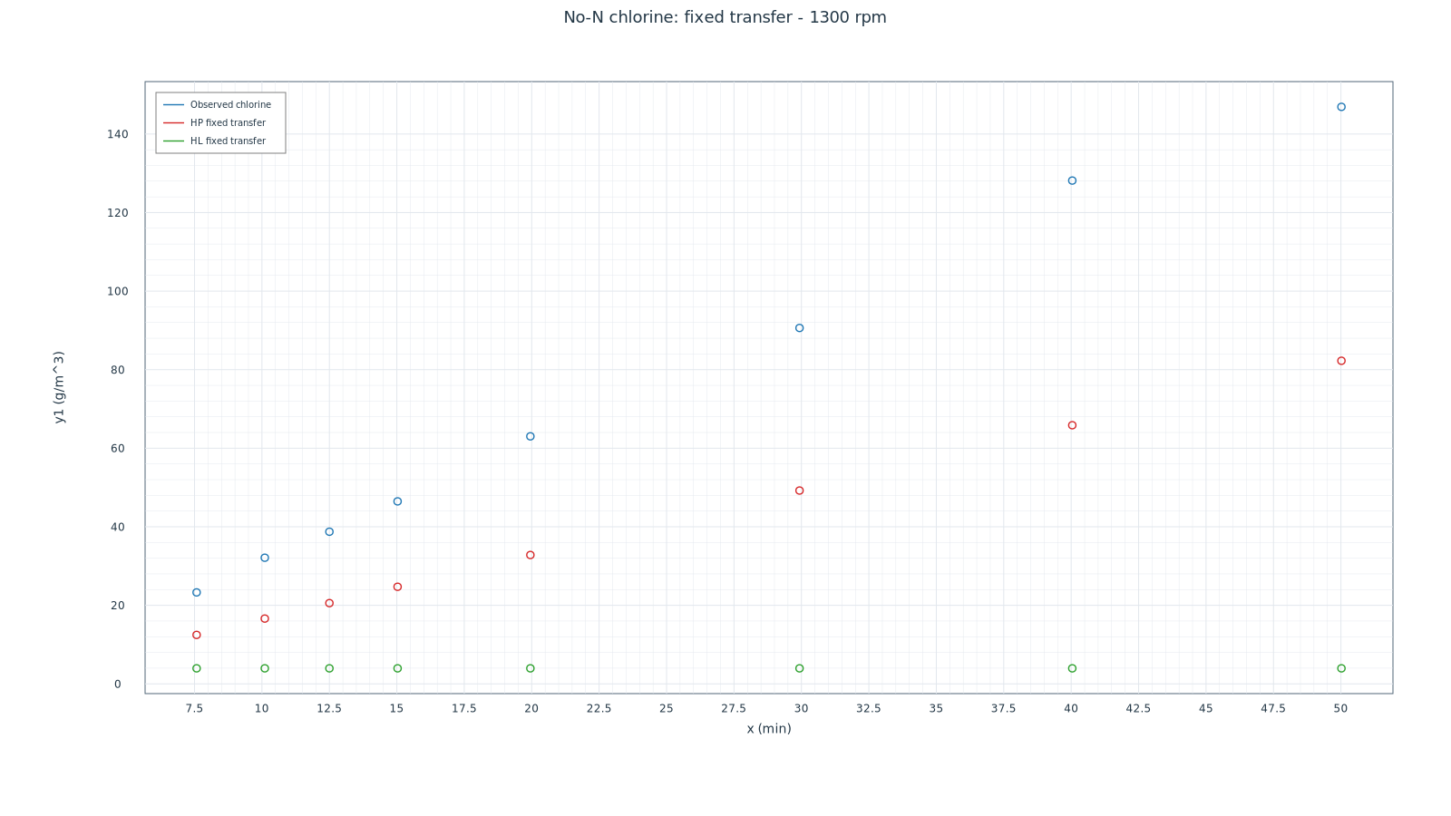
About 147 mg Cl₂/L observed, versus 82 and 4 predicted. At 1300 rpm and around 50 minutes, the nitrogen-free control accumulated much more chlorine than either model calibrated on the nitrogen curves predicted. A model can fit the nitrogen signal and still fail to predict the chlorine concentration in a separate trial.
How does faster stirring change the ammonia signal?
We started with the measurements of Atrashkevich and colleagues and reconstructed the published curves at 0, 100, 500 and 1300 rpm in GX-TXT. Although faster stirring can improve transport, the analytical signal associated with ammonia can fall more slowly in this experiment. Stirring changes transport to the electrodes and interfaces and can also change the amount of oxidant available to react with nitrogen. To distinguish these explanations, we compared the nitrogen assay, chlorine measured in nitrogen-free trials and bulk pH.
The nitrogen assay provides the data for the fits. The DPD chlorine control tests hypotheses about oxidant availability. Bulk pH constrains the distribution of species under the adopted equilibrium assumptions. Each measurement constrains a different part of the problem.
From the nitrogen signal to a two-pool model
The model uses two concentrations: the nitrogen pool A associated with the assay response (mol N/m³), and the accessible oxidant pool B (mol Cl₂ equivalent/m³). The source P depends on current I, volume V, the Faraday constant F and an operational factor f. The coefficient κ describes effective oxidant loss. The coefficient ν is the oxidant demand per unit of nitrogen consumed in the model.
The product AB represents the effective coupling between the pools. With a constant source and no initial oxidant, the balance allocates the supplied oxidant among the amount still available, the amount consumed with nitrogen and the amount lost. The DPD assay and gross anodic efficiency each require their own observables.
A better fit still leaves a pattern in the residuals
For the four S2 calibrations, we fixed the net chlorine accumulation rates reported for the nitrogen-free trials and fitted only the reactivity parameter h. Net accumulation falls from 6.6 to 2.9 mg Cl₂/L/min between 0 and 1300 rpm. The fitted h falls at 100 rpm, rises at 500 rpm and falls again at 1300 rpm. The series offers no evidence of a monotonic relation between reactivity and stirring speed.
| Stirring (rpm) | Net S2 accumulation without N (mg Cl₂/L/min) | Fitted h | RMSE (mg N/L) |
|---|---|---|---|
| 0 | 6.6 ± 0.3 | 0.05865 | 0.339 |
| 100 | 5.9 ± 0.3 | 0.03928 | 0.213 |
| 500 | 3.6 ± 0.2 | 0.07607 | 0.474 |
| 1300 | 2.9 ± 0.2 | 0.00774 | 0.754 |
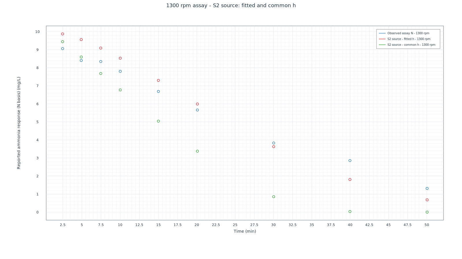
At 1300 rpm, fixing h at its 0 rpm value drives the predicted nitrogen signal almost to zero near 50 minutes, when the digitized observation is still about 1.31 mg N/L. Fitting h reduces RMSE from 1.768 to 0.754 mg N/L. At both 500 and 1300 rpm the errors still have a temporal pattern. The model tends to overestimate the signal initially and underestimate it toward the end.
The nitrogen-free control tests both hypotheses
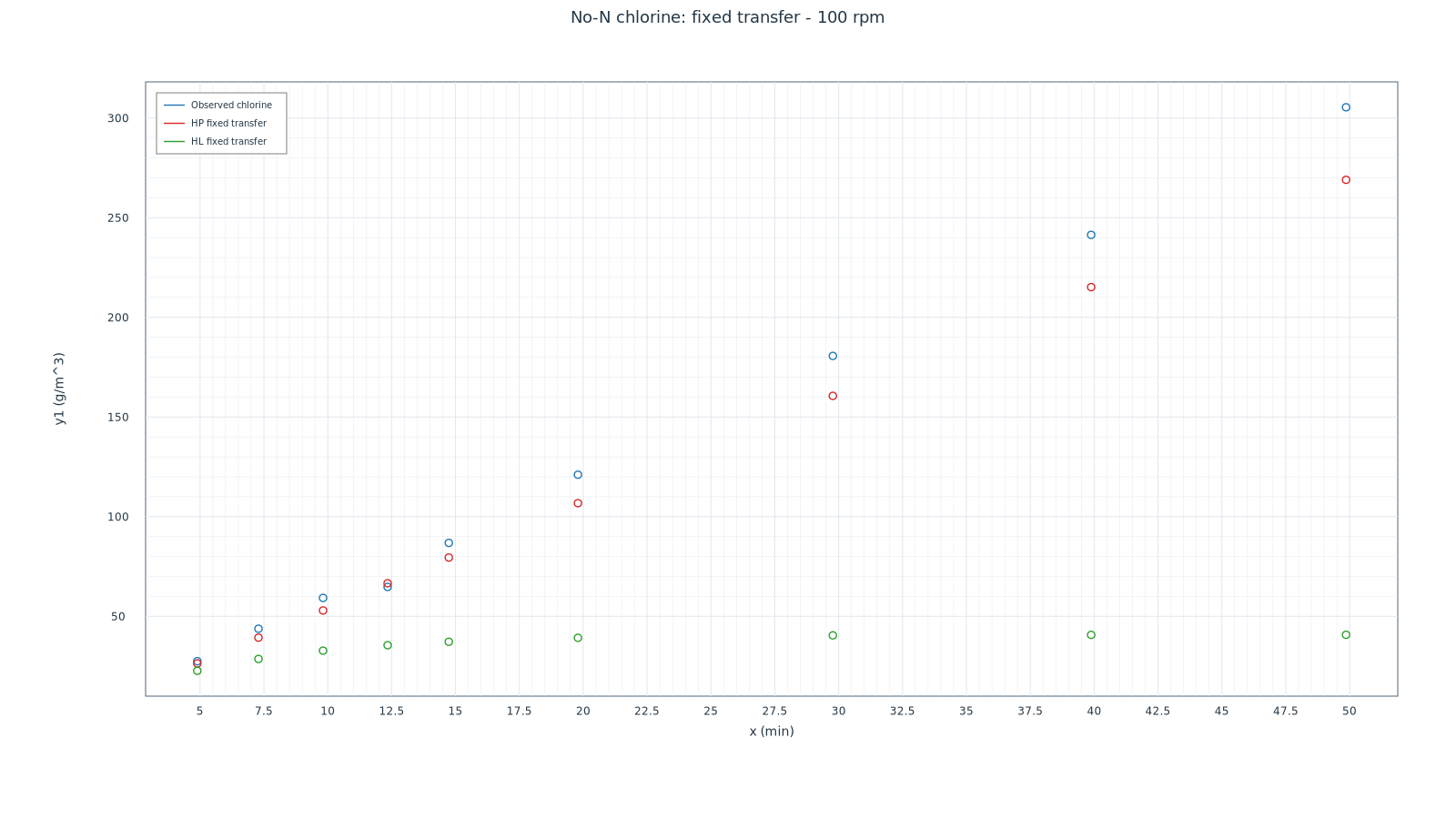
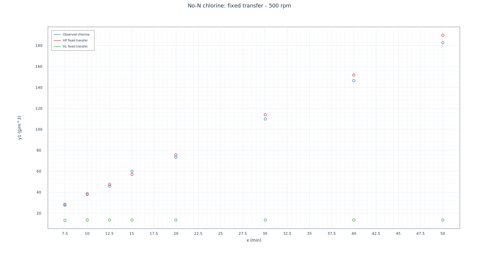
We built two operational explanations. HP varies the oxidant source and sets loss to zero. HL varies the loss and keeps the reference source. After fitting the nitrogen curves, we evaluated each hypothesis at the observed times of the nitrogen-free trials, keeping its parameters fixed. The six predictions test whether the same explanation holds when the control measures chlorine alone.
At 100 rpm HP increasingly underestimates accumulation. At 500 rpm it follows the control more closely, with late deviations. At 1300 rpm both predictions lie below the observations. HL describes the nitrogen curves at high stirring rates but predicts an almost flat chlorine curve. The discrepancy challenges the transfer of a single loss coefficient across the two types of trial.
The current ceiling and the chlorine deficit
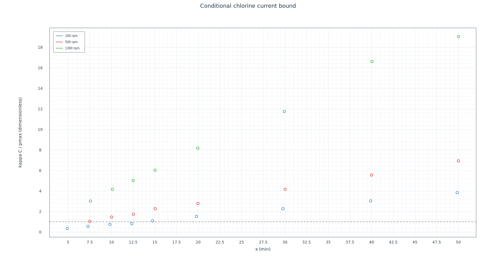
We compared predicted loss κC with the maximum chlorine source allowed by the current, pmax. Their ratio cannot exceed one if the source stays below that ceiling, loss is first order and the initial concentration is below the corresponding threshold. With the transferred coefficients, 21 of 25 points nominally exceed one. The final point at 1300 rpm reaches about 19.05. The points belong to three time series and the value closest to one is sensitive to uncertainty. The large late discrepancy, especially at 1300 rpm, is the strongest test of the model.
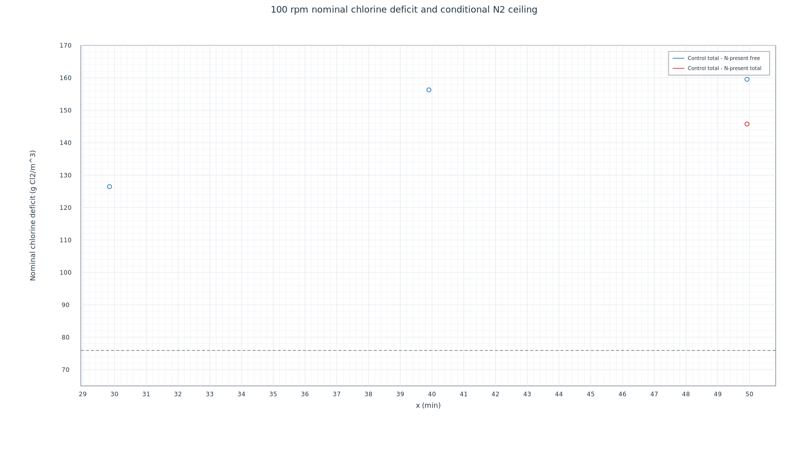
The 100 rpm experiments provide a second constraint. We compared three free-chlorine points and one late total-chlorine point. The total gives a nominal deficit of about 146 mg Cl₂/L, roughly 70 mg Cl₂/L above the ceiling for the N₂ endpoint under the shared-source and shared-loss assumptions. The total is more informative than free chlorine alone because chloramine formation can lower free chlorine while retaining chlorine in the system. The late point is a single digitized marker in an area of overlap and supplies no independent confirmation of the free-chlorine comparison. The balance tests the assumptions jointly and leaves the final nitrogen pathways open.
What bulk pH adds
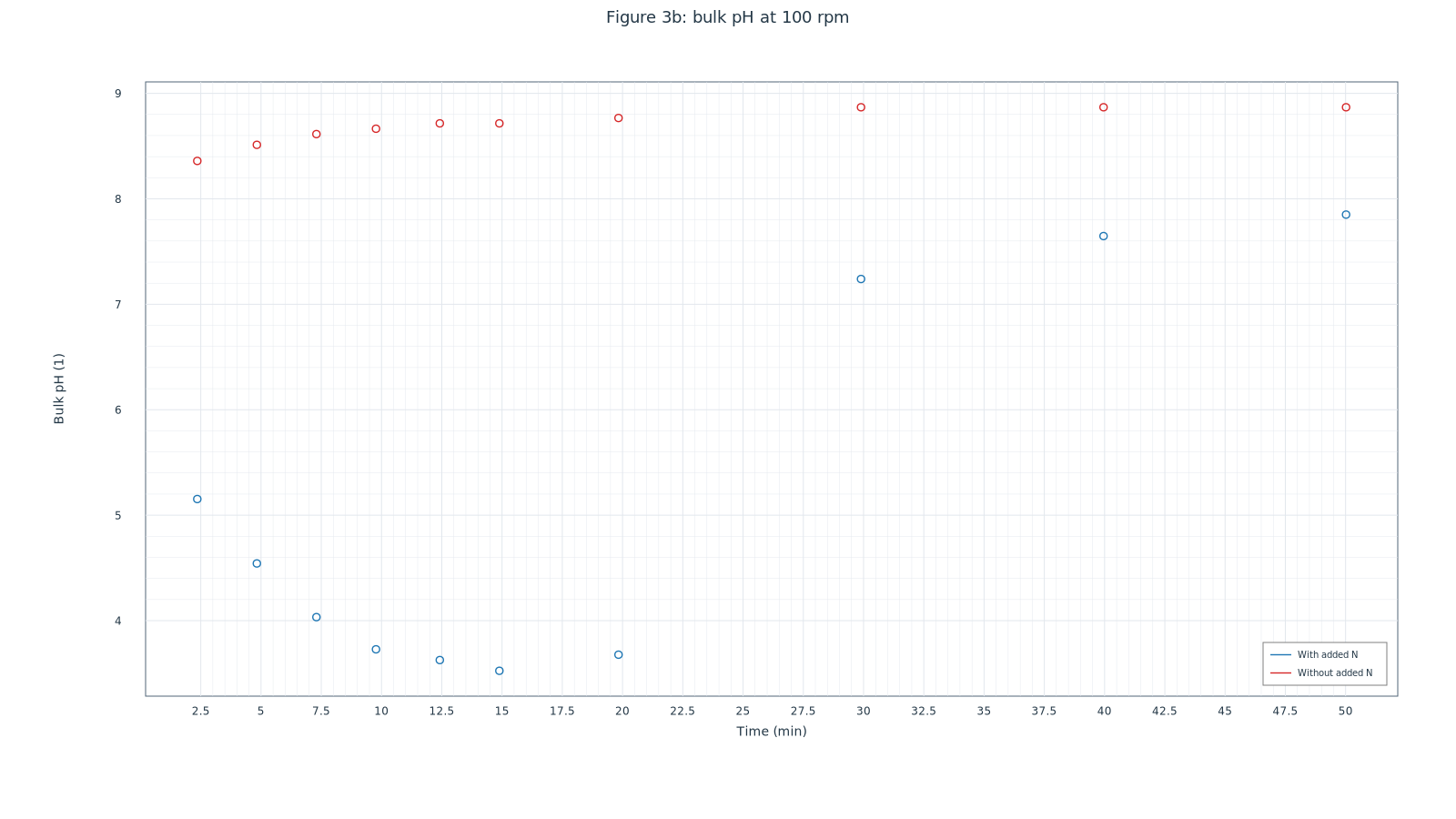
At 100 rpm we digitized ten points from each bulk pH trace, with and without nitrogen. For the nitrogen-present trace we used GX-TXT to calculate the ideal NH₃ fraction and the conditional fractions of dissolved Cl₂, HOCl and OCl⁻. Bulk pH comes from the observations and the fractions follow from the assumed equilibrium model. Connecting either fraction to a loss rate requires another equation. How much nitrogen escaped as NH₃ and how much oxidant was transformed or lost remain open questions.
Where the investigation stopped
The comparisons indicate that chlorine production, transformation and transport must be distinguished. Our analysis began to converge on an approach already represented in the literature, and we stopped developing the model. Romano, Ortiz and Urtiaga provide a methodological comparison by calibrating the source separately and accounting for chloramines and the balances. Their experimental conditions differ. ELEC shows where the two operational hypotheses cease to hold simultaneously for this dataset and which measurements could better distinguish them.
The ELEC project diary
- ELEC 01 — What does the experiment measure? Nitrogen, chlorine and pH
Why does the ammonia-related signal fall more slowly at higher stirring rates? We examine what the nitrogen and chlorine assays measure and what bulk pH and electrode transport can tell us. - ELEC 02 — Model hierarchy: effective kinetics, transfer and identifiability
A two-pool model separates oxidant supply, effective reactivity and loss. Native GX-TXT calibrations and an analytical solution show when the nitrogen curves can identify those contributions. - ELEC 03 — From fits to constraints: what does the chlorine balance reveal?
Two hypotheses can fit the same nitrogen signal and still predict very different chlorine levels. We test them against nitrogen-free controls, the Faradaic ceiling and the paired chlorine deficit. - ELEC 04 — Kinetics, speciation and transport: from local reaction to reactor response
Bulk pH, equilibrium speciation and reaction times help distinguish rapid local chloramination from the slower response observed in the stirred reactor. - ELEC 05 — Gas loss, chloramines and the proton balance
How much ammonia transfer to the gas would explain the falling nitrogen signal? Chlorine and proton balances constrain stripping, chloramine storage and other possible nitrogen pathways. - ELEC 06 — Where the numbers came from: GX-TXT, GNU Octave and reproducibility
Follow the results back to native GX-TXT jobs at 0 and 100 rpm, the original GNU Octave scripts, the output tables and the checks still outstanding. - ELEC 07 — Sources, conclusions and tests that could distinguish the mechanisms
Which explanations for the effect of stirring survive all the comparisons? We review the original sources, the GX-TXT results and the measurements that could distinguish the remaining hypotheses.
How we used GX-TXT
In a single session we gathered the sources, calibrated the figures with Curve Digitalizer and published the curves as Datasets with units and provenance. We fitted the nitrogen curves with Curve Fitter and used the Worksheet for the current-ceiling comparisons. GNU Octave scripts and native GX-TXT jobs integrated the operational network at 0 and 100 rpm and produced nine tables for each case. The diary links the model, balances and calculations to the relevant datasets.
Sources and related reading
- Atrashkevich et al. (2025) — Water Research
Source of the experimental curves, trial conditions and chlorine controls. - Romano, Ortiz and Urtiaga (2021) — Comprehensive kinetics of electrochemically assisted ammonia removal
Published model that treats the chlorine source, chloramines and balances separately. - Qiang and Adams — Monochloramine formation kinetics
Reference for the HOCl–NH₃ reaction and pH sensitivity. - Jafvert and Valentine (1992) — Chlorination kinetics
Successive reactions and rate-law conventions. - Gendel and Lahav (2012) — Electrochemical chlorination
Hydrolysis, chloramines and interpretation of UV and DPD measurements. - Zhang et al. (2018) — Water Research
Reaction scheme and limits of kinetic closures. - Sander (2023) — Compilation of Henry’s law constants
Henry-law conventions and the distinction between neutral and total species. - Clegg and Brimblecombe (1989) — Solubility of Ammonia
Ammonia solubility, concentration and activity conventions. - Degermenci (2022) — Air stripping of ammonia using a gas-liquid contactor
Forced-air stripping in a gas–liquid contactor. - Corruchaga et al. (2022) — Ammonia evaporation
Evaporation of ammonia from aqueous solutions exposed to wind. - Hossini et al. (2016) — Optimizing ammonia volatilization by air stripping
Forced stripping as a function of pH, dose and airflow. - Hasar et al. (2009) — Leachate treatment
Application of stripping in a multistage process. - Connick and Chia (1959) — The Hydrolysis of Chlorine
Reference on hydrolysis, temperature and activity. - Aieta and Roberts (1986) — Henry constant of molecular chlorine
Reference on the solubility of molecular chlorine in water. - Whitney and Vivian (1941) — Solubility of Chlorine in Water
Reference on the solubility of chlorine in water. - Turbulence and electrical resistance in single-phase electrolytes
Giux-Lab article on the role of flow in electrochemical response. - Electric field line distortion in electrochemistry
Giux-Lab article on current distribution, transport and resistance.
Software used
- GX-TXT Source and dataset management, digitization, curve fitting and scientific computing.
Project log 7
- Nov 20, 2026 ELEC 02 — Model hierarchy: effective kinetics, transfer and identifiability A two-pool model separates oxidant supply, effective reactivity and loss. Native GX-TXT calibrations and an analytical solution show when the nitrogen curves can identify…
- Nov 20, 2026 ELEC 03 — From fits to constraints: what does the chlorine balance reveal? Two hypotheses can fit the same nitrogen signal and still predict very different chlorine levels. We test them against nitrogen-free controls, the Faradaic ceiling…
- Nov 20, 2026 ELEC 01 — What does the experiment measure? Nitrogen, chlorine and pH Why does the ammonia-related signal fall more slowly at higher stirring rates? We examine what the nitrogen and chlorine assays measure and what bulk…
- Nov 20, 2026 ELEC 07 — Sources, conclusions and tests that could distinguish the mechanisms Which explanations for the effect of stirring survive all the comparisons? We review the original sources, the GX-TXT results and the measurements that could…
- Nov 20, 2026 ELEC 04 — Kinetics, speciation and transport: from local reaction to reactor response Bulk pH, equilibrium speciation and reaction times help distinguish rapid local chloramination from the slower response observed in the stirred reactor.
- Nov 20, 2026 ELEC 06 — Where the numbers came from: GX-TXT, GNU Octave and reproducibility Follow the results back to native GX-TXT jobs at 0 and 100 rpm, the original GNU Octave scripts, the output tables and the checks…
- Nov 20, 2026 ELEC 05 — Gas loss, chloramines and the proton balance How much ammonia transfer to the gas would explain the falling nitrogen signal? Chlorine and proton balances constrain stripping, chloramine storage and other possible…