

ELEC 02 — Model hierarchy: effective kinetics, transfer and identifiability
A two-pool model separates oxidant supply, effective reactivity and loss. Native GX-TXT calibrations and an analytical solution show when the nitrogen curves can identify those contributions.
Two pools with explicit units
The accepted operational model uses seconds, constant volume and two concentrations: A in mol N/m³ and B in mol Cl₂-equivalent/m³. Its equations are
The retained parameter pack has I=0.12 A, V=0.0002 m³ and F=96485.33212 A·s/mol. Two electrons correspond to one Cl₂ equivalent. The initial state is A₀=(10 g N/m³)/M_N, M_N=14.0067 g/mol, and B₀=0. The definition k_A=h/(A₀τ), with τ=6 s, gives k_A in m³/(mol·s), dimensionless h and κ in s⁻¹. The six-second quantity is a normalization, not a measured mixing or residence time. A plotted minute coordinate and the registered second-based model must be connected through their actual unit contract.
A is an analytical pool and B an accessible oxidant pool. Their product is an effective closure, not a claim that the elementary HOCl+NH₃ reaction directly removes the assay pool. h is not a converted fraction, collision probability or tracer mass-transfer coefficient. Its declared interval [0,1] is the domain of this parameterization, not a universal chemical bound. Because k_A=h/(A₀τ), changing A₀ at fixed h also changes k_A: that would not be an initial-concentration experiment at fixed intrinsic kinetics.
The operational oxidant inventory is
The minus sign matters: consuming A also demands oxidant. This is a pool ledger under ν, not a complete elemental and charge balance for the electrolyte. The ν=1.5 conditional N₂ endpoint and historical ν=4 nitrate scenario remain distinct. Neither is a measured product yield.
Different calibrations answer different questions
The earlier zero-rpm reference related a source fitted to the nitrogen-free chlorine control to the nitrogen response. From this reference, H_P varies f with reference reactivity and zero loss; H_L varies κ with reference source and reactivity. Six genuine native calibrations establish their conditional responses. Their different flexibility is not an automatic selection of CER change versus cathodic reduction.
The S2 branch instead fixes κ=0 and ν=1.5, imposes each RPM’s reported mean net nitrogen-free rate, and fits only h. Native unit-aware conversion uses f=2FVp/(M_Cl₂I), with M_Cl₂=70.906 g/mol. S2 is net accumulation, not gross anodic generation. Its estimator and time window are incompletely specified. Treating it as a constant zero-loss source in a nitrogen-present experiment is a calibration convention. Adding a loss without reconsidering that source would change the meaning of the control.
| rpm | S2 p, mg Cl₂/L/min; reported SD | Native fixed f | Native fitted h | N RMSE, mg N/L |
|---|---|---|---|---|
| 0 | 6.6; 0.3 | 0.4989416285034647 | 0.0586539723742101 | 0.33855343638612906 |
| 100 | 5.9; 0.3 | 0.4460235769955215 | 0.03928129500594746 | 0.21260451565227792 |
| 500 | 3.6; 0.2 | 0.27214997918370804 | 0.07607195484315359 | 0.47426242309268246 |
| 1300 | 2.9; 0.2 | 0.21923192767576477 | 0.007743099116693341 | 0.7544382681368795 |
Long decimals provide machine-record reproducibility, not experimental accuracy. No confidence intervals or propagation of digitization and S2 uncertainty were produced. All fitted h values lie inside their declared bounds. Their nonmonotone ordering does not establish a monotone RPM–transport law. Structured residuals remain at 500 and 1300 rpm: too much nitrogen signal predicted early and too little late. A local objective minimum is not proof of chemical adequacy or a global optimum. Complete S2 interpretation.
The common-h control transfers the actually fitted zero-rpm S2 h while keeping RPM-specific S2 f. Its native RMSE values are 0.46897, 0.49968 and 1.76830 mg N/L at 100, 500 and 1300 rpm; allowing h to vary gives 0.21260, 0.47426 and 0.75444. At 500 rpm the improvement is modest and does not prove kinetic equality. At 1300 rpm common h removes the late signal too quickly: at 50.037 min it predicts about 0.0000587 against 1.3140 mg N/L observed. Freeing h improves error without automatically repairing shape. This constrains the transferred-source/constant-reactivity closure rather than identifying a new reaction.
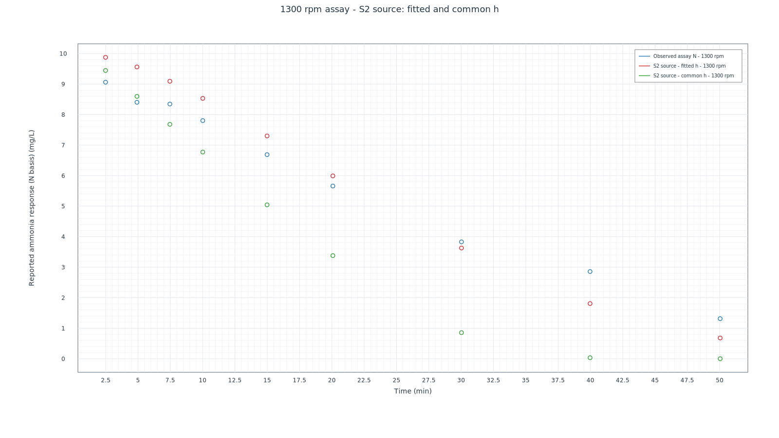
Native graph p0029 compares assay-N observations, the conditional fitted response and the common-h control. Connecting computed samples does not create additional observations. Better fit and explained mechanism remain different conclusions.
A precise identifiability result
Writing q=−A′/A=k_AB gives q′=k_AP−(νk_AA+κ)q. An ideal continuous response could identify α=k_AP, β=νk_A and γ=κ if the regressors 1, Aq and q are independent. For known positive ν and nonzero k_A, k_A=β/ν and P=αν/β. The initial product k_AP therefore does not prove universal structural non-identifiability.
If ν is unknown, the transformation k_A→s k_A and (P,ν,B)→(P,ν,B)/s leaves A unchanged. The adopted observation model then has a scale ambiguity. Even where ideal coefficients are identifiable, six to nine points do not yield accurate derivatives. Noise, time origin, B₀ and recovery limit practical inference. No observed curves were differentiated. Identifying coefficients would still not identify the physical origin of κ. Analytical note.
Analytical verification and actual native integration
For κ=0, substitute B=Pt+νA−νA₀ and z=1/A. Then z′=k_A(Pt−νA₀)z+k_Aν. With q₀(t)=k_A(Pt²/2−νA₀t),
This checks numerical execution without adding a physical hypothesis. The accepted stable formulation uses scaled functions and limiting cases; positive κ uses the existing public ODE owner. The native reaction-network module 0.2.5 genuinely executed the same zero-rpm operational case: two species, seven parameters, three channels, 61 times over 0–1200 s and nine canonical tables. Its ode45 state comprises amounts in mol plus three reaction extents, five states in total. AbsTol=10⁻¹⁰ applies in that basis, not directly to mol/m³.
An external independent verification of the existing native arrays, using high-accuracy quadrature of the analytical solution, found maximum absolute errors about 1.3531×10⁻¹³ for A and 2.0304×10⁻¹³ for B in mol/m³. Maximum relative errors were about 1.18×10⁻¹² and 4.59×10⁻¹², excluding B₀=0 from the relative denominator. This is verification of native production, not an externally produced scientific trajectory. The near-machine linear-inventory residual, about 2.22×10⁻¹⁵, would not alone establish global accuracy.
The actual 100-rpm parameter variant also completed through native 0.2.5: 151 retained times over a declared 0–3000 s theoretical grid and nine tables. Its saved model owner is at revision 4. The original nitrogen-calibration window remains 2.3743325716139645–19.843825433296708 min. Later theoretical output is temporal extrapolation beyond that calibration, even when a software query-domain flag reports no extrapolation relative to its supplied chlorine coordinates. No residual metric was manufactured by interpolating observations onto the uniform grid. Dedicated generic-network figures are not claimed; older Fitter figures are not relabelled as these new solves.
Datasets
S2 calibrations and common-h controls · Operational0rpm network: nine outputs · Operational100rpm network: nine outputs · Original assay-N centres
Digitized Figure 3 observations (12 CSV files in a ZIP archive) · Native model and constraint results (27 CSV files in a ZIP archive)
Other steps of this project
- ELEC 03 — From fits to constraints: what does the chlorine balance reveal?
- ELEC 01 — What does the experiment measure? Nitrogen, chlorine and pH
- ELEC 07 — Sources, conclusions and tests that could distinguish the mechanisms
- ELEC 04 — Kinetics, speciation and transport: from local reaction to reactor response
- ELEC 06 — Where the numbers came from: GX-TXT, GNU Octave and reproducibility
- ELEC 05 — Gas loss, chloramines and the proton balance