

Vibration After an Impact
Use the measured hammer force to locate the impact. Follow the accelerometer response, compare sections of the decay and use a periodogram to identify prominent frequency bands.
Impact test and unit conversion
Saullo G. P. Castro, Delft University of Technology, Impact hammer test of an Aluminium 6082 T6 plate, 260 × 246 × 1.5 mm, free boundary conditions (2023), CC BY 4.0. The plate was suspended on soft cotton threads to approximate free edges. Impact point 13 is at (0.130, 0.123) m and the single-axis accelerometer is fixed at point 5 at (0.260, 0) m in the author’s XY coordinate system. The selected file is Waveforms Point13.tdms, group Configuration0_Impact00. Zenodo record and protocol · Original TDMS file
force_n- Hammer load cell channel
cDAQ1Mod1_ai0, in N. accel_m_s2- Synchronized channel
cDAQ1Mod1_ai1, converted from g to m/s² with the author’s factor of 9.81. time_s- Derived from the common
wf_incrementof 0.0001171875 s. The sample rate is 8,533.333… Hz. All 32,768 samples are retained. Time zero is the maximum absolute force, at zero-based index 9. The preceding segment contains 9 samples, about 1.05 ms. The file records 8 pretrigger samples relative to its own trigger, which differs from the selected force maximum.
Quality check, envelope and periodogram
- Import the Dataset. In Signal Analysis, choose
plate_impact, setaccel_m_s2as the primary signal andtime_sas the time coordinate. Leave Paired blank and the declared rate at0. - Click Analyze with
quality.basic. Readn,peak,rmsandcrest_factorin the report. This method produces a scalar summary. - Switch to
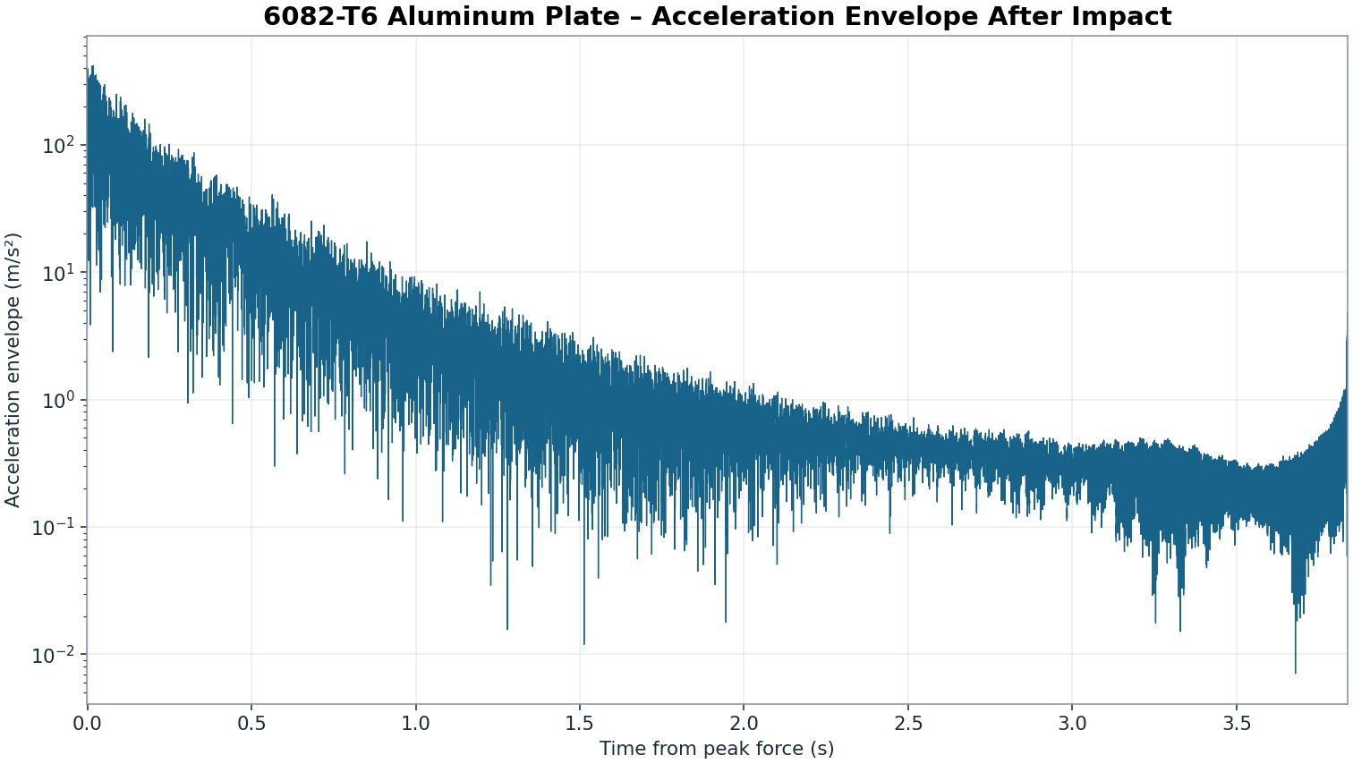
analytic.envelope, click Analyze and publish with an unused ID, for examplereal.plate.envelope.amplitudestill uses m/s². Compare sections of the decay on the same scale. - Choose
spectral.periodogram, click Analyze and publish withreal.plate.periodogram. The full-record FFT has 32,768 points, 0.2604167 Hz bin spacing and 16,385 one-sided bins up to about 4,266.67 Hz. The Hamming window weights the start and tail differently. Use the peaks as indications of frequencies present in this transient record.
Read the decay and frequency peaks
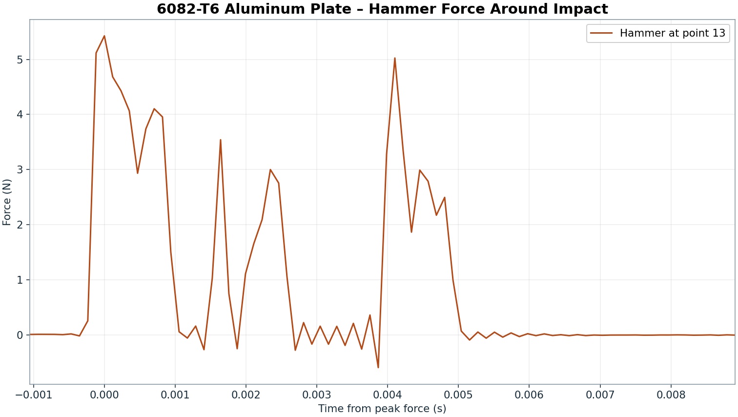
The summary reports an absolute peak acceleration of about 397.23 m/s², RMS of about 21.39 m/s² and a crest factor of about 18.57. The crest factor expresses the large difference between the peak and the RMS level of the full recording. The synchronized force trace locates the excitation. It has several lobes in the first few milliseconds, including a local peak of about 5.03 N at +4.10 ms. The first window used to compare the decay starts at +20 ms, after the strongest force lobes. The acceleration is still oscillating in this window.
| Window after peak force | Envelope RMS (m/s²) | dB relative to the first window |
|---|---|---|
| [0.02, 0.07) s | 149.10 | 0.00 |
| [0.50, 0.55) s | 16.94 | −18.89 |
| [2.50, 2.55) s | 0.43 | −50.77 |
The four highest local peaks in the periodogram are at about 1,214.32, 972.14, 740.10 and 360.16 Hz, in descending PSD order. The reference results include the full frequency grid.
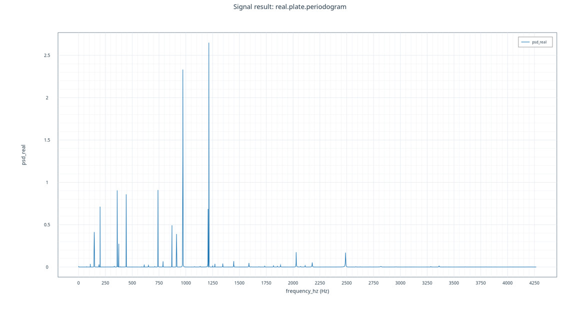
The observed frequencies characterize this particular impact and sensor pair. Modal characterization and frequency response function (FRF) estimation would require dedicated measurements and analysis, including several comparable impacts. This exercise uses a single recording with a force of finite duration. When interpreting the peaks, consider the measured shape of the excitation and the location of the sensor. CC BY 4.0, attributed to Saullo G. P. Castro