

Interpret FEM Results and Repeat the Exercises
Inspect verified results
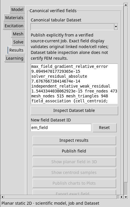
With a COMPLETED job associated with the correct revision, open Results and press Inspect results in the tab or menu. The result fills a read-only pane. Scroll to see numerical checks, units and a preview of up to 20 cells. Draft changes do not affect the completed job. Save the revision you want to study and start a new Run FEM to get its results.
- solver_residual_absolute
- Norm of the residual of the system assembled by GetDP. It also depends on the scale of the system.
- independent_relative_weak_residual
- Dimensionless relative residual reconstructed independently on the actual free degrees of freedom. Like the GetDP residual, it checks the discrete solution. To assess physical accuracy, also compare with a reference and vary the mesh size.
- max_field_gradient_relative_error
- Maximum relative discrepancy between the vector field and the gradient of the nodal potential, with the derivative and sign determined by the selected physics.
- free_nodes, mesh_nodes and mesh_triangles
- Number of free nodes, total number of nodes and number of triangles in the computed mesh. Use the counts to compare two discretizations.
- kind, job_id, state, solver_versions, native_sha256
- Model type, job ID and state, tool versions and hash of the native component. Use these details to distinguish runs.
- node_potential_unit, field_unit and field_association
- Units of the nodal potential and field, and the field’s association with the original cells. The preview shows connectivity through the three node IDs and lists field values. The cell column
potentialcontains the mean of the triangle’s nodal potentials.
Electrostatic exercise
In a fresh window, choose electrostatic_2d. Set Half domain width (m) to 0.05, Full domain height (m) to 0.1, εr to 1, the right boundary potential to 10 V and the mesh size to 0.005 m. If you started with New electric, overwrite the suggested dimensions, potential and mesh size. You can also download the scientific model and import it as described in the chapter on Workspaces. Press Validate, Run FEM and Status, then Inspect results when the calculation finishes.
Under these ideal conditions, w = 0.05 m and V(x) = 10(x + w)/(2w). The electric field E = −∇V is uniform, with Ex = −100 V/m and Ey = 0. Compare the sign of field_x, the value of field_y and the magnitude field_norm on the cells. The reference run reports about 515 nodes and 948 triangles. The color scale can make rounding differences look larger.
analytic_max_relative_field_error gives the maximum relative discrepancy from the ideal field. analytic_area_rms_relative_field_error gives the area-weighted relative root-mean-square discrepancy. In the test case they are approximately 2.7 × 10⁻¹⁴ and 5.3 × 10⁻¹⁵, respectively. The reference is the ideal rectangle with the prescribed boundary conditions.
Magnetostatic exercise
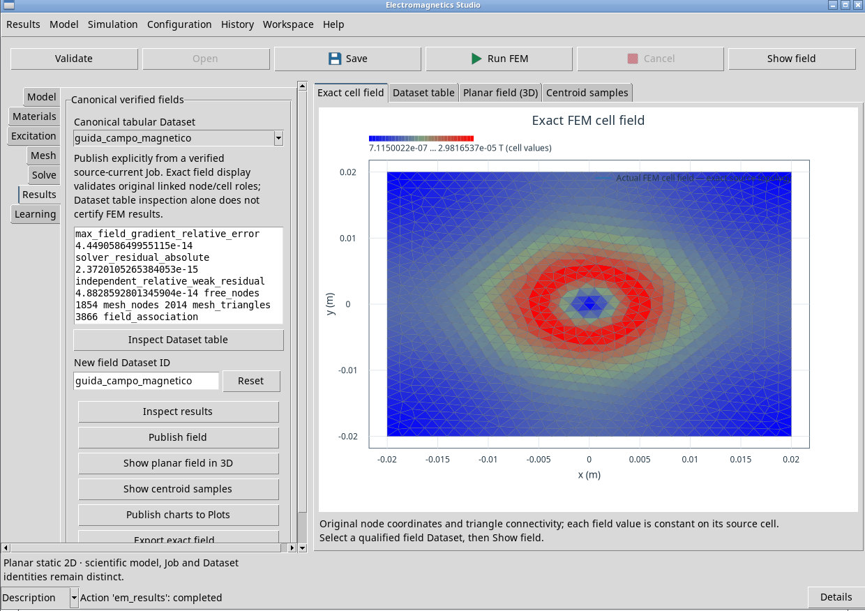
Use New magnetic. Set the half-width to 0.02 m, height to 0.04 m, conductor μr to 1, radius to 0.005 m, Jz to 10,000 A/m² and mesh size to 0.0015 m. Set Model ID to a value such as guida_conduttore. Validate the model and run the job. The model solves for the axial potential Az in Wb/m and computes the magnetic field B in tesla from its curl.
In the reference case with μr = 1 and unbounded air, I = Jzπa² ≈ 0.785398 A. Inside the disk, Bθ = μ₀Jzr/2. Outside, Bθ = μ₀I/(2πr). The tangential component is positive in the direction associated with positive Jz. The actual rectangle imposes Az = 0 on its boundary, so local comparisons near the edge are affected by the finite domain.
- mesh_current_A and nominal_circle_current_A
- Current from the actual triangulated area of the conductor and current for the ideal disk. Approximating the circular boundary can cause a difference.
- ampere_loop_T_m, ampere_mesh_expected_T_m and ampere_mesh_relative_error
- Numerical circulation of B in T·m around a circle of radius 1.5a, reference value μ₀ times the current represented by the mesh, and relative error between the two. Keep the ideal current and the current through the triangulated area distinct when comparing the numbers.
Compare two computed meshes
Keep the first result and note its IDs. Change only the mesh size to 0.001 m and start a new Run FEM. You can also duplicate the scientific model to keep two independent copies. In Inspect results, compare the quantities at the same geometry and source settings.
| Mesh size (m) | Nodes | Triangles | Mesh current (A) | Circulation (T·m) | Relative circulation error |
|---|---|---|---|---|---|
| 0.0015 | 1018 | 1926 | 0.776457 | 9.5418 × 10⁻⁷ | 2.208% |
| 0.001 | 2014 | 3866 | 0.780361 | 9.7865 × 10⁻⁷ | 0.202% |
In these two runs, the finer mesh reduced the discrepancy. Repeat the comparison for each new model and observable. Both exercises use linear, static, planar 2D physics and explicit boundary conditions.