

How temperature changes the 1N4148 diode’s I–V characteristic
How much does a 1N4148’s forward voltage change as its junction gets hotter? At 1 mA, I obtained about 0.607 V at 25 °C and 0.368 V at 150 °C from Vishay’s typical curves. A difference of nearly 0.24 V shows why it is worth specifying both current and temperature. I digitized three curves in GX-TXT and compared the Shockley model with a version that includes series resistance. The residuals show where in the current range that resistance makes a difference.
From the datasheet to 146 points
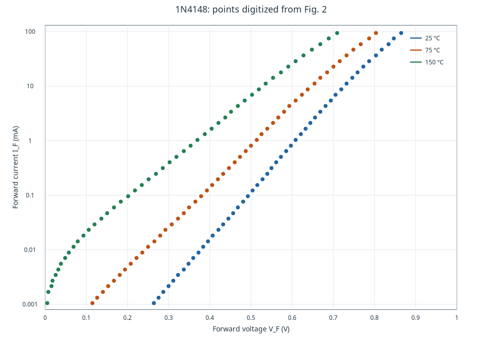
I used Figure 2 on page 2 of Vishay datasheet 81857, revision 1.6, dated 7 November 2024. In Curve Digitalizer I calibrated the four corners of the chart. The horizontal axis runs linearly from 0 to 1 V. The vertical axis runs logarithmically from 0.001 to 100 mA. A check at the nominal grid intersection (0.4 V, 1 mA) returned 0.399 V and 1.013 mA. I used this comparison to check the calibration at that grid point. The reading is limited by the resolution of the chart and the position of the click. Vishay datasheet, p. 2.
I rasterized the panel with Poppler at 288 dpi. I located the center of each colored trace at roughly 11-pixel intervals along Y and placed those points in Curve Digitalizer. The near-uniform Y spacing gives nearly uniform sampling in log-current.
The plot below uses the same variables as the original Figure 2, so I can compare the slopes and horizontal separation of the traces. I kept blue for 25 °C, orange for 75 °C and green for 150 °C. The family published by GX-TXT contains 49, 49 and 48 points respectively, spanning about 0.00105 to 93.7 mA at all three temperatures. The legend gives \(T_j\), the junction temperature, which can differ from ambient temperature, including through self-heating. Original Figure 2.
How much the voltage falls at fixed current
I interpolated voltage between the two adjacent samples as a function of \(\log I_F\). The currents 0.1, 1 and 10 mA are inside all three curves. I calculated the secant slope between 25 and 150 °C. It is less negative as current increases over the sampled range. At 1 mA the two partial secants are −1.89 and −1.93 mV/°C. I treat these as interval averages because three temperatures do not establish a local derivative.
| IF (mA) | 25 °C (V) | 75 °C (V) | 150 °C (V) | 25–150 °C secant (mV/°C) |
|---|---|---|---|---|
| 0.1 | 0.494 | 0.381 | 0.205 | −2.32 |
| 1 | 0.607 | 0.512 | 0.368 | −1.91 |
| 10 | 0.727 | 0.647 | 0.529 | −1.58 |
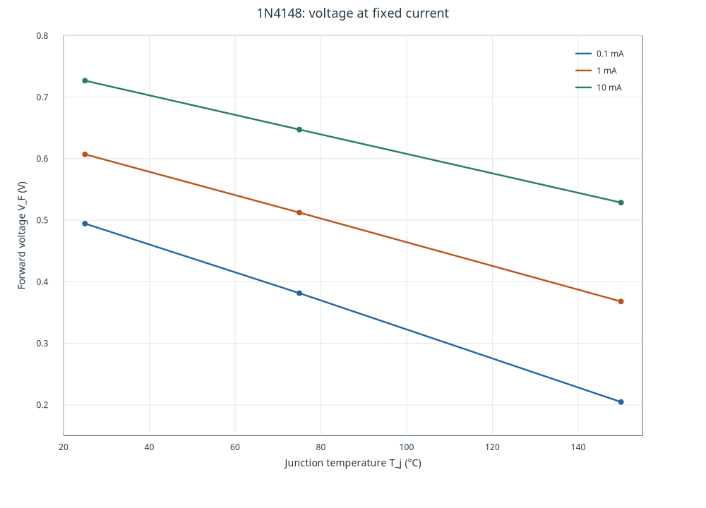
Figure 1 in the same Vishay datasheet (p. 2) plots \(V_F\) directly against \(T_j\) at fixed current. On visual comparison, it shows the same curve ordering and negative slopes. The table uses interpolation from Figure 2 alone. I left out 100 mA because it is above the last digitized point. Datasheet Figure 1.
Two models for the junction
A forward-biased PN junction conducts when the applied voltage reduces the barrier to carrier transport. In the Shockley model, \(I_S\) sets the current scale, \(n\) is the ideality factor, and \(V_T\) is the thermal voltage. With series resistance, \(I_F R_s\) accounts for part of the voltage across the terminals.
\[ \begin{aligned} I_F &= I_S\left[\exp\!\left(\frac{V_j}{nV_T}\right)-1\right] \\ V_T &= \frac{k_B T_j}{q} \\ V_F &= V_j+I_F R_s \end{aligned} \]
\[ V_F(I_F)=nV_T\ln\!\left(1+\frac{I_F}{I_S}\right)+I_F R_s. \]
I fitted voltage at the currents of the original points. The inverse equation is explicit even with series resistance, so I could minimize the sum of squared voltage residuals with equal weight per point. I converted current to amperes, temperature to kelvin for \(V_T\), and constrained \(R_s\geq0\). A logarithmic display axis changes the presentation. The objective still uses voltage. That choice matches the question about forward drop at a set current. Estimates depend on the residual variable and the fitted interval.
I used Python Script inside GX-TXT to search for the minimum over \(\ln I_S\), solving the linear coefficients at each step. I repeated the full-domain fits in Curve Fitter with the same formula and the Ceres solver. All six converged and their RMSEs agree to the reported precision. For the base model I fixed \(R_s=0\). The table gives the full-domain parameters. Lines in the graphs join model predictions at the original currents.
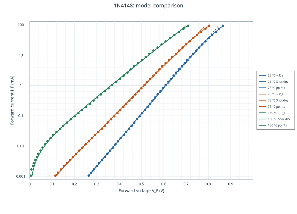
| Tj (°C) | Model | IS (nA) | n | Rs (Ω) | RMSE (mV) |
|---|---|---|---|---|---|
| 25 | Shockley | 6.6 | 2.000 | 0.000 | 5.28 |
| 25 | Shockley + Rs | 5.3 | 1.948 | 0.339 | 1.41 |
| 75 | Shockley | 176 | 1.987 | 0.000 | 5.04 |
| 75 | Shockley + Rs | 157 | 1.946 | 0.294 | 2.53 |
| 150 | Shockley | 6961 | 2.016 | 0.000 | 4.10 |
| 150 | Shockley + Rs | 6663 | 1.991 | 0.136 | 3.69 |
The fitted \(I_S\) increases enough with temperature to outweigh the rise in \(V_T\). That helps explain the lower voltage at the same current over the range studied.
Where series resistance helps
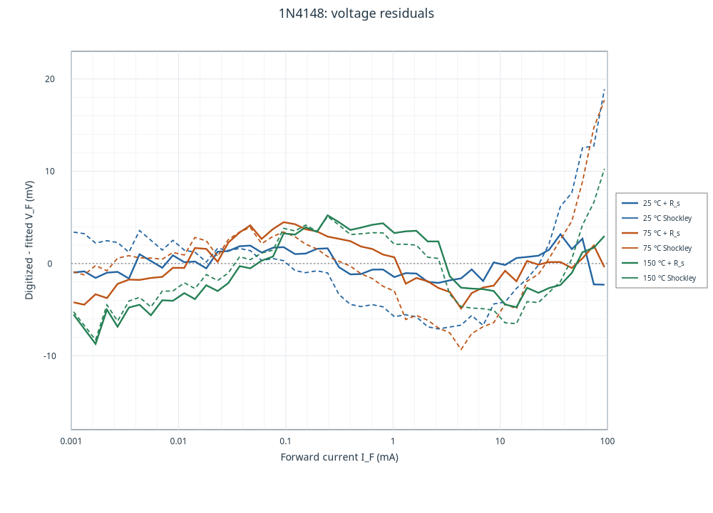
At 25 °C, adding \(R_s\) reduces the RMSE from 5.28 to 1.41 mV. Above 10 mA it drops from 8.97 to 1.84 mV, consistent with the \(I_F R_s\) contribution. At 75 °C the overall RMSE drops from 5.04 to 2.53 mV. At 150 °C the gain is smaller, from 4.10 to 3.69 mV. At that temperature the series term reduces high-current errors, but below 0.01 mA the RMSE increases from about 5.00 to 5.62 mV. I define residuals as digitized voltage minus fitted voltage.
I repeated the comparison with just the 29 points per curve from 0.01 to 10 mA. Shockley alone gives an RMSE of 1.13, 1.74 and 2.79 mV. With the series term at 75 and 150 °C, the optimum in that central range is at the constraint \(R_s=0\). At 25 °C the estimate changes from about 0.34 Ω over the full range to 0.45 Ω in the central range, with a local gain of just 0.18 mV. I therefore use series resistance mainly to describe the upper-current range and treat \(I_S\), \(n\) and \(R_s\) as effective fitted parameters.
Resolution and limits of the comparison
Line thickness, raster resolution and the four calibration references limit point reading. One horizontal pixel in the working plot is about 1.7 mV. This quantifies geometric resolution. Estimating a standard deviation would require an error model. Calibration errors can move many points in the same direction. Residuals against these typical curves do not establish production spread or a confidence interval for the component. Thermal dynamics, capacitance, reverse current and behavior outside the sampled interval require separate data or models.
The RMSEs compare models on the same points used to estimate their parameters. Evaluating predictions for other devices or conditions would require independent data.
To estimate \(V_F\) from 0.01 to 10 mA, the simpler model describes these data within a few millivolts. At higher current I prefer the series-resistance model, especially at 25 and 75 °C. I specify both current and junction temperature when comparing an operating point with the datasheet.
Reproducing the analysis
I used GX-TXT DEV112 P011-bis, Curve Digitalizer 2.0.26, Dataset Curve Fit 0.46.2, and Curve Viewer 2.0.0 with the Native2D renderer. I published the accepted calibration as a numerical family in the Session. The CSV retains curve and point identities, indices, raster coordinates and calibrated values. The script reads that family within Python Script, publishes the derived series and prints the report. The plots come from Curve Viewer.
The Curve Fitter text reports record the solver comparison. Convergence means the solver met its stopping criteria. The physical interpretation also depends on the residuals and on how estimates change with the fitted interval.
Repeating the fit in Curve Fitter
For each junction temperature I select the corresponding input (diode_25_fit_input, diode_75_fit_input or diode_150_fit_input). I set X to forward_current in A and Y to forward_voltage in V. In Safe formula… I enter a*log(1+x/s)+r*x with orientation Y = f(X) and zero shifts. Here a is in V, s in A, and r in Ω. For the Shockley fit I fix r=0. For the version with series resistance I let r vary with a lower bound of zero.
Download the canonical CSV for all three curves · Download the data, results and Python script (.zip). The archive includes the CSV, the numerical report risultati.json with the fit ranges, and analisi_1n4148.py for the GX-TXT Python Script module.
References
Vishay Semiconductors, 1N4148, document 81857, revision 1.6, 7 Nov 2024, p. 2, Fig. 1 and Fig. 2.
From the same category
- The 2D21 Thyratron: From Historical Curves to SPICE Models
- Zenith Flash-Matic Receiver: Circuit Analysis
- GX Whiteboard Studio: a Debian digital whiteboard for recording lessons, the complete manual
- GX-TXT Temporal Set API: Managing Time Segments and Windows with GNU Octave and Python
- Turbulence and Electrical Resistance in Single-Phase Electrolytes: When Flow Changes the Electrochemical Response
- Electric Field-Line Distortion in Electrochemistry: Turbulence and Resistance