GX-TXT: Your Experiment and Your Project in One Integrated Environment

The problem: experimental data get lost along the way

Anyone who takes measurements in a lab knows the scene. Raw data sit in one folder, scripts in another, plots are exported as images, the fit was done in yet another program and the notes are in a notebook or a text file. Every hop from one tool to the next is an export and an import, and every hop loses something: units, the variable name, the filter that was applied, the excluded point, the script version.

A few months later, looking at a plot, the question “exactly which data does this curve come from?” often no longer has a reliable answer. GX-TXT was built to answer that question at any time.

Why I built it

GX-TXT grew out of my own experimental work, not out of a whiteboard idea. At first I wanted something simple: put my scripts in order, stop losing data along the way and stop rewriting the plotting code every time. The first core came from tests on an infrared remote control: signals to acquire, analyse and compare. From there the need widened to measurements, fits, historical curves to digitize, and geometry built on top of the data.

No tool I knew held all of this together without losing the link to the original data. So I started building one. I am its first user: every tool you find inside exists because I needed it for my work.

What GX-TXT is: many tools, one environment

GX-TXT is an integrated environment for managing an experiment and the project that contains it, from data acquisition to results. It brings together tools that usually live in separate programs:

• a spreadsheet for tabular data;
• scientific curve editors: the digitizer, the Curve Workbench, the Interactive Builder, the fitter;
• analysis modules — statistics, spectra, replicate analysis and much more — around a hundred in the current version;
• Python and GNU Octave scripts (Octave is compatible with MATLAB syntax);
• interactive 2D and 3D plots and a 3D editor;
• acquisition and import from instruments, files, audio, images and documents.

The interface is written in Tcl/Tk, computation runs through GNU Octave and Python, and geometry is handled by native engines in C and C++. It is free software, released under the GNU GPL version 3 or later. The current version is a beta: more on that below.

Project and experiment: the data stay together

The point I built everything around is organization. In GX-TXT, work has three levels:

• Project: the container that groups related experiments, with name, description, tags and author;
• Experiment: the scientific identity of the study, with its own notebook — objective, procedure, observations, operator, date, notes;
• Session: the operational, reproducible record, which keeps configuration, Datasets, source files, notes, registered scripts, analyses, plots and provenance.

A Project organizes without duplicating: attaching an experiment to a project neither copies nor moves its data, and detaching it deletes nothing. A Session can be exported in portable form and reopened elsewhere with its identities intact. The details are in the Projects, Experiments and Sessions guide (currently in Italian).

Every piece of data is a canonical Dataset, organized in namespaces, with variables that carry a stable identifier, a unit and their metadata. You can attach notes and metadata to anything — a dataset, a curve, a plot. When a tool produces a result, that result is a new Dataset that carries its origin with it: source, filters, parameters.

The original data are never modified, and every result can be traced back to what it came from. So, months later, you reopen the project and find not just the numbers but also how you got there.

Behind this sit a few principles that recur across the whole system:

• Canonical Datasets: tools work on registered identities and scientific metadata, not on files picked ad hoc by the code;
• Public APIs: scripts and modules access Datasets, plots, selections and persistence through versioned contracts;
• Session and provenance: configurations, sources, scripts and results stay linked to the work that produced them;
• Separation of computation and presentation: scientific data stay distinct from plots and viewers;
• Extensibility: Python, GNU Octave and installable modules let you go from exploration to distribution without modifying the CORE.

An example: from an old datasheet to curves with their uncertainty

The 2D21 is a thyratron, and its original datasheet is a scanned PDF: the characteristic curves — grid current versus grid voltage, for several anode currents — exist only as a drawing. Here is how they become data with their uncertainty, without leaving GX-TXT.

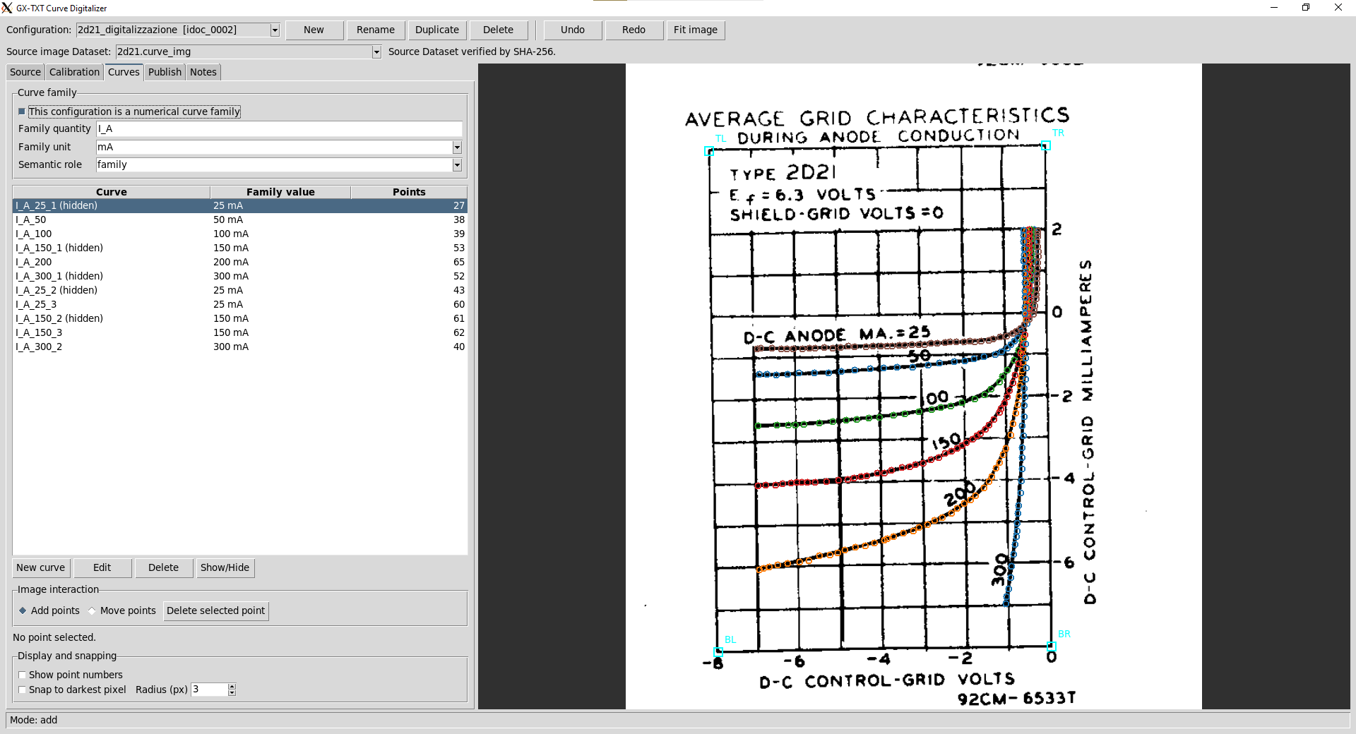
1. Digitization. The datasheet image enters the project as a Dataset, verified with SHA-256. In the Curve Digitizer I calibrate the axes on the four corners of the chart and define the curve family: the family quantity is the anode current I_A, in mA, with one curve per value (25, 50, 100, 150, 200 and 300 mA). I digitized some of the curves several times, on purpose.

2. Replicate analysis. The repeated digitizations become separate Datasets. The Replicate Curve Analysis module combines them and produces, for each curve of the family, a consensus curve with its uncertainty, separating the contribution of repetition within the same source from the differences between sources.

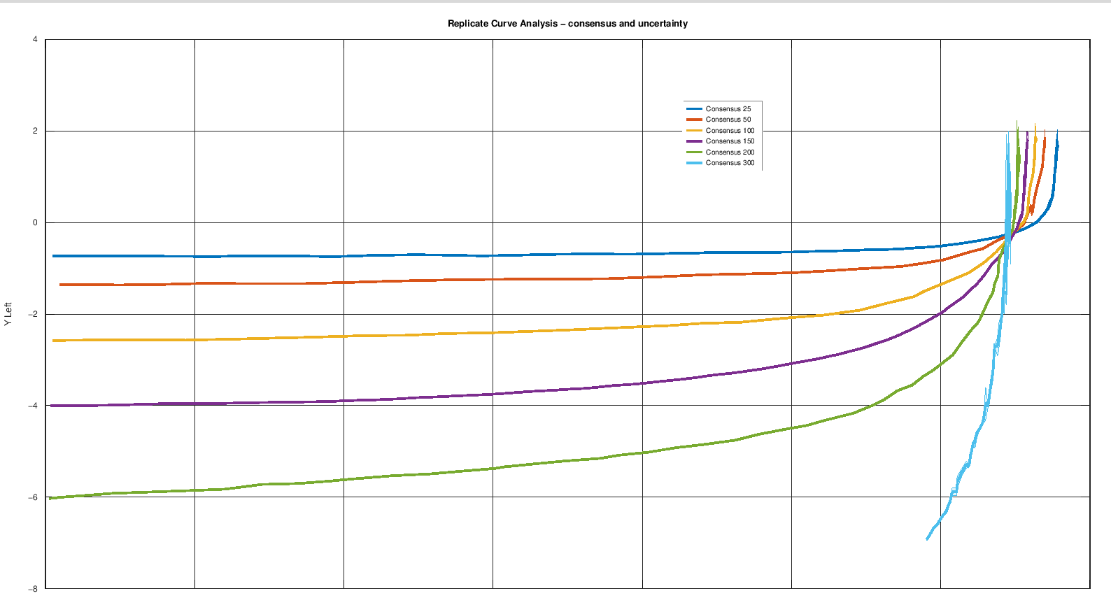
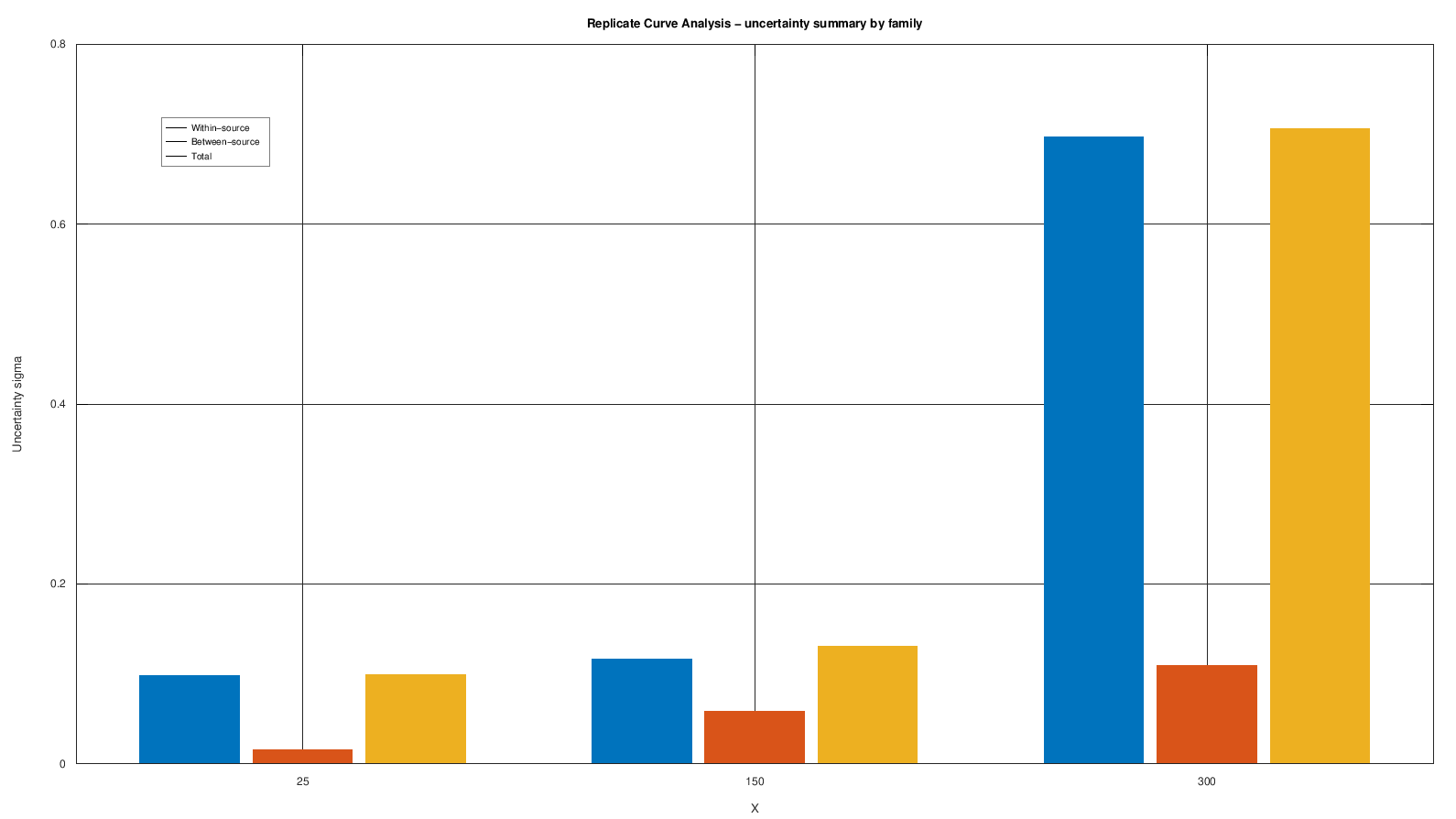
The result shows something you cannot see by eye: the uncertainty is small on the nearly horizontal stretches and jumps where the curve becomes nearly vertical, because there a tiny error in the voltage read moves the current a lot. For the 300 mA curve the total uncertainty is about seven times that of the 25 mA curve.

3. Fit. The curves move on to the fitter with their provenance intact: every parameter stays traceable to the original datasheet, the calibration and the replicates used. Each step produces a Dataset with its own metadata and notes, in the same project.

From measurement to model: Dataset Curve Fit

The fitter works directly on a Dataset: you choose the dataset, the X and Y variables, optional filters (expressions too, handy when working with curve families), then the model. The flow is always the same: fit preview, check, and only at the end Accept, which publishes the result as a new curve with its provenance.

The models available today range from linear and polynomial to exponential, power law and Gaussian, up to smoothing splines, PCHIP, Fourier series, arcs, Bézier curves and parametric models. The orientation can be chosen (Y = f(X), X = f(Y), parametric, polar), so curves that are not functions can be handled correctly too.

Below the plot are the residuals, point by point, in the original units. It is my favourite part: the fit itself tells you where the model fails.

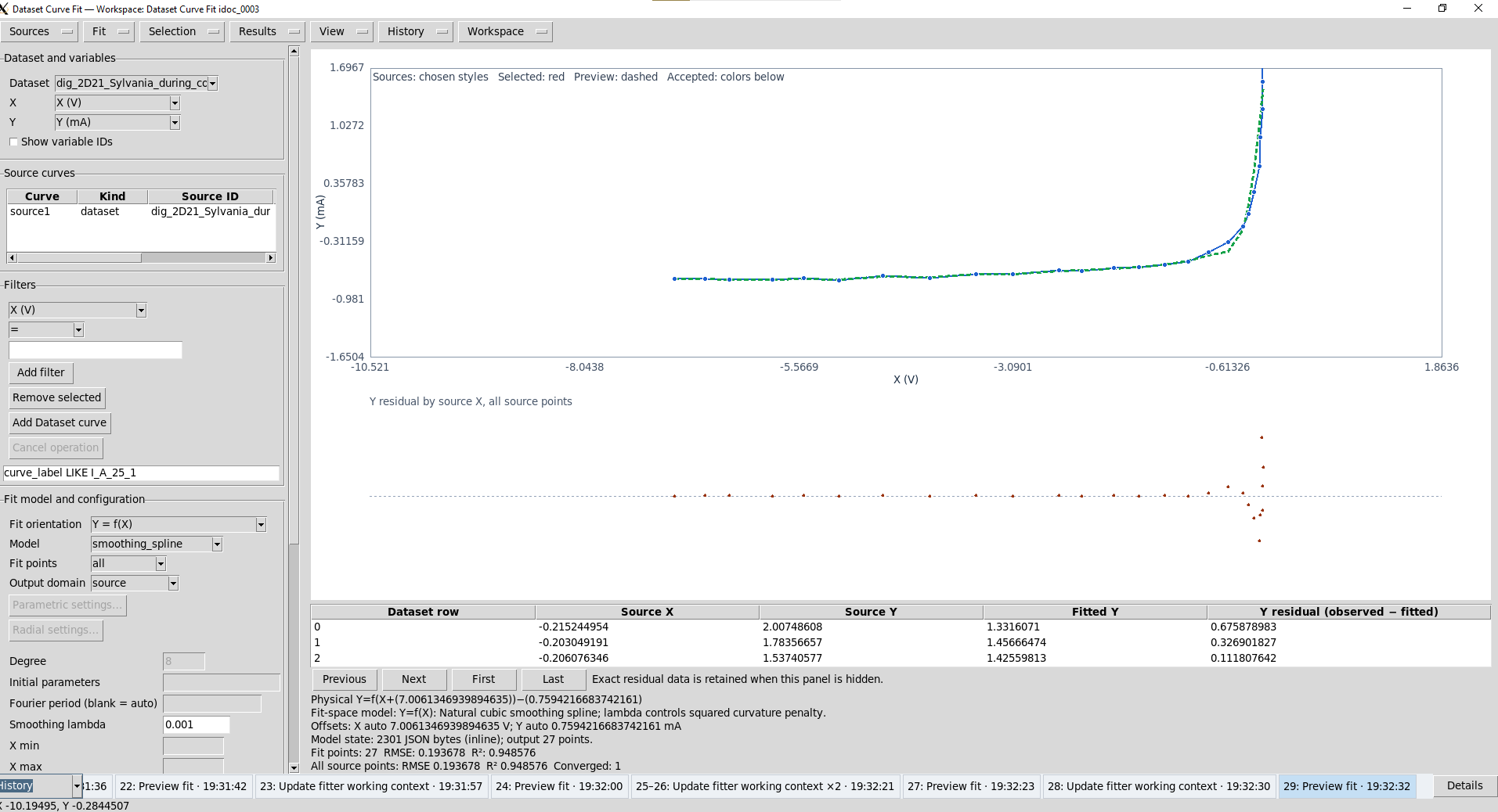
The fitter is the part I am working on most right now. Since this is a beta, much will arrive in the next versions: more models, complete statistics and parameter uncertainties, a more polished interface.

Curve Workbench: experimental data and geometry together

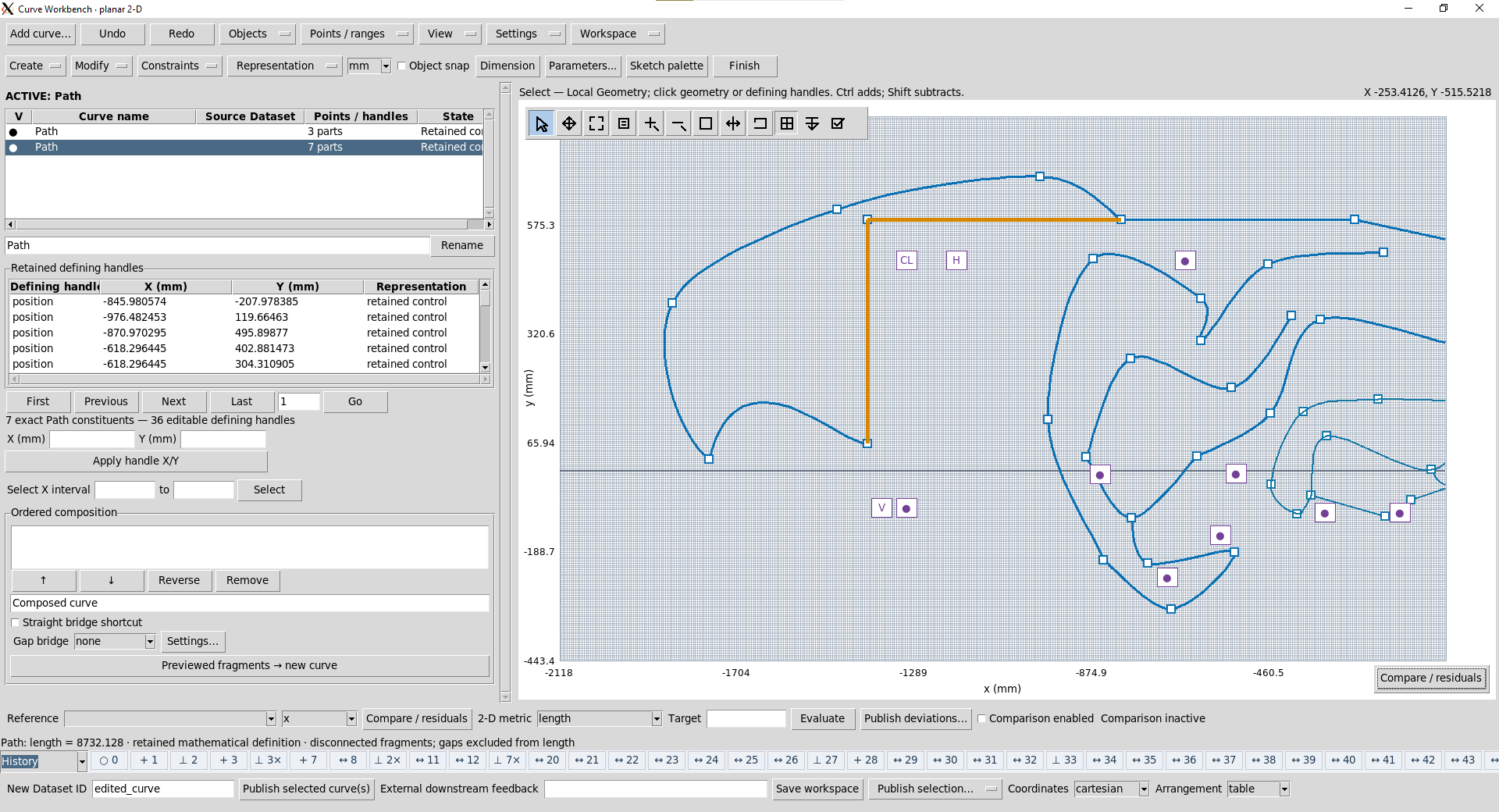
The Curve Workbench is a workbench for curves. It is not a CAD program, even though it has much of what you would expect from a 2D CAD: lines, arcs, circles, splines, Bézier curves, constraints, dimensions, snapping, numeric editing of control points. The difference is the purpose: here geometry lives alongside experimental data, and the two always stay distinct. Being a geometric tool, with rotations, symmetries and distances, it works best when X and Y share the same unit: profiles, contours, sections, paths. For curves linking different quantities, such as a voltage and a current, the right tools are the fitter and the Interactive Builder.

A curve that comes from a Dataset keeps its exact points and its provenance. On top of it you can draw your own constructions: tangents, reference lines, approximations. And you can ask the tool how far your construction departs from the measured data, with Compare / residuals. Classic graphical methods done by eye thus become graphical methods with a measured error.

A dataset can be converted into geometry and geometry into a dataset. Every conversion creates a new object: the original data stay where they are, and the derived object remains recognizable as such.

Interactive 3D plots and native geometry

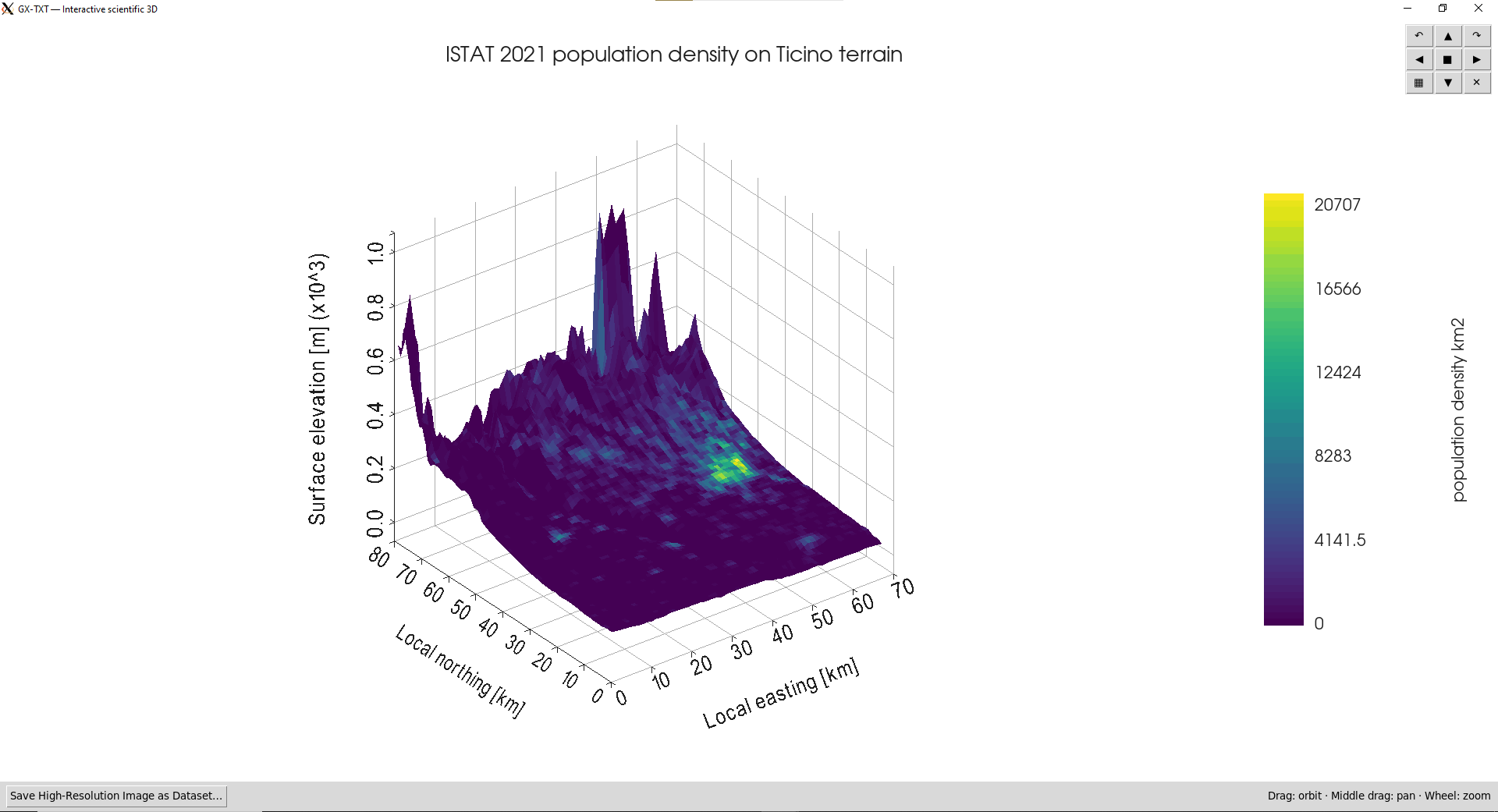
Dataset 3D plots are truly interactive: they open in a separate window and can be rotated, panned and zoomed. In the geospatial demo, for example, the terrain elevation of the Ticino valley forms the surface and ISTAT 2021 population density provides the colour. Even the high-resolution image you export from it is saved as a Dataset, with its provenance.

Underneath there are two native geometry engines: a 2D one written in C and a 3D one in C++. The 3D APIs are already quite advanced; the 3D geometry viewer, on the other hand, is still young and I am completing it. I keep the two apart in the documentation too: 3D data plots work today, the viewer for 3D geometry is on its way.

Python and Octave scripts: two examples

If you prefer writing code, you give up nothing. Python and GNU Octave scripts are registered in the Session and work through the same public APIs used by the graphical tools: they read and publish Datasets, use the numerical functions and create plots. A result obtained from a script has the same provenance as one obtained from the interface.

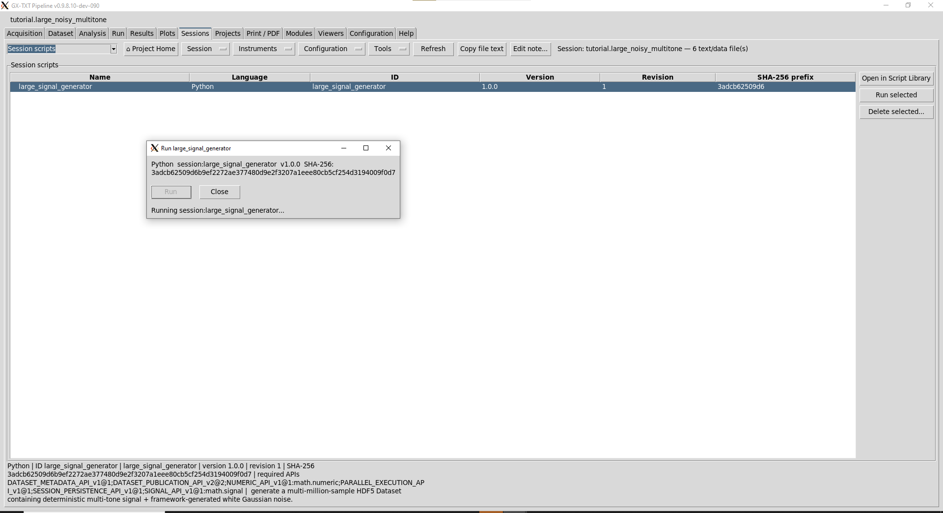
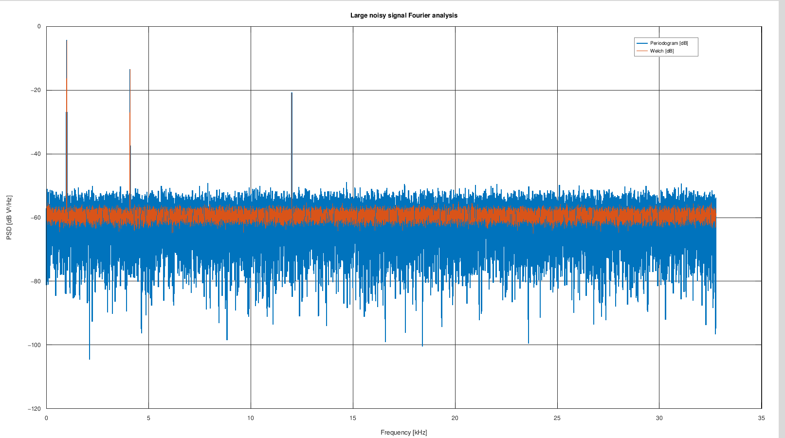
Large Datasets, Fourier and parallel computing. One script generates a 4,194,304-sample signal — three tones at 997, 4,093 and 12,011 Hz plus white noise — and publishes it as an HDF5 Dataset in about 3 seconds. A second script reads it in chunks and computes its statistics without loading it all into memory. A third computes the periodogram and the Welch estimate and creates a persistent plot in the Session. A fourth compares serial and parallel FFTs on four processes, with a speedup of about 2.4×.

STFT and reconstruction. The second example starts from a non-stationary signal of 131,072 samples: a chirp from 100 to 3,000 Hz, white noise and two impulses at 4 and 11 seconds. The script computes the short-time Fourier transform through the framework APIs and keeps it whole, as a complex matrix in a two-dimensional HDF5 Dataset: 2,048 frequencies by about 513 time frames. It then inverts it and reconstructs the signal with a root-mean-square error of the order of 10⁻¹⁶ V, that is, at machine precision. Window, hop and NFFT are stored in the metadata, and every derived Dataset points back to the original one.

In both cases the results are Datasets with their metadata, available to the other tools: no script writes private files or images on its own.

Features are organized into installable modules. The APIs are documented as versioned contracts, about sixty documents, so anyone writing a module knows exactly what they can rely on.

Where things stand

The version published today is a beta, 0.9.8.10-dev-095. It works and I use it every day, but it is not the final version yet: the interface changes often, some internal flows are being rewritten and plenty of polishing is still to come.

Coming in the next versions:

• a rewritten internal data flow and a much expanded fitter, with statistics and parameter uncertainties;
• the complete 3D geometry viewer;
• new scientific libraries;
• CFD trajectory handling and a viewer for preparing OpenFOAM dictionaries;
• documentation and tutorials redone on the stable version.

I am not giving dates: the first stable version will come out when it has everything it needs and the tests pass. Until then I will publish further betas, clearly marked as such.

How to try it

The source code is on GitHub: giuxlab-hub/GX-TXT. The documentation, still under construction and currently in Italian, is at gxtxt.giux-lab.it.

What you need:

• Linux (the bundled native libraries target Linux);
• Tcl/Tk with wish for the interface;
• GNU Octave and Python 3 for the scientific modules and scripts, plus the dependencies of the modules you use (NumPy, SciPy, Matplotlib and others).

Start it with wish gxtxt_pipeline.tcl. It is a source distribution, not an installer: for now it is best to try it on a test Session, not on important data.

If you try it, I would like to know what works, what breaks and what is missing for your work.

The first of a series

This article only gives an idea. In the next ones I will go into the individual tools: digitization and replicate analysis, the fitter, Python scripts on large Datasets, spectral analysis, 3D plots.