6BX7-GT: SPICE Model, Koren Fitting and Validation
The 6BX7-GT is a twin triode used in the receiver of the Zenith Flash-Matic, the visible-light wireless television remote control introduced by Zenith in 1955 and designed by Eugene J. Polley. In the original circuit, the 6BX7-GT is used in the section that controls the motor and relays employed for channel selection.
A technical reconstruction of the Flash-Matic therefore requires not only studying the original schematic, but also sufficiently reliable models of the active devices used in the receiver. This is the motivation for the work described in this article: to build a SPICE model of the 6BX7-GT from the plate characteristics published by General Electric and to determine its validity range quantitatively.
The resulting model describes the static plate characteristic Ia = f(Va, Vg). It is therefore not intended to represent the complete physical behavior of the tube: in the version presented here, grid current, interelectrode capacitances, the heater, and other dynamic effects are not modeled. The objective is instead to provide a verified static representation that can be used in SPICE with explicitly known accuracy and limitations.
Original General Electric datasheet
The primary reference used to build and validate the model is the original General Electric 6BX7-GT datasheet.
Download the original General Electric 6BX7-GT datasheet
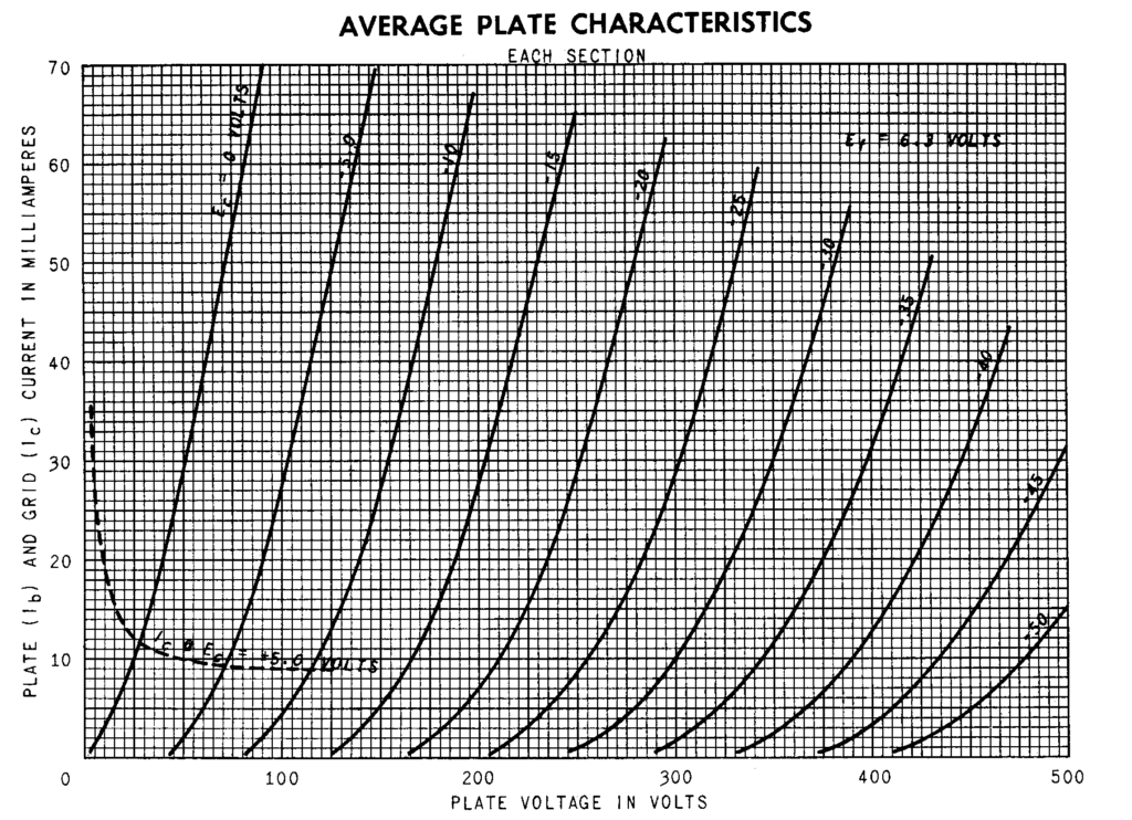
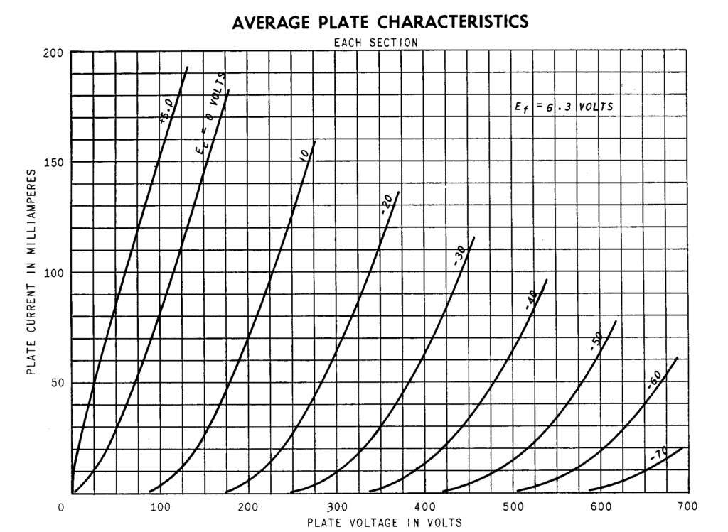
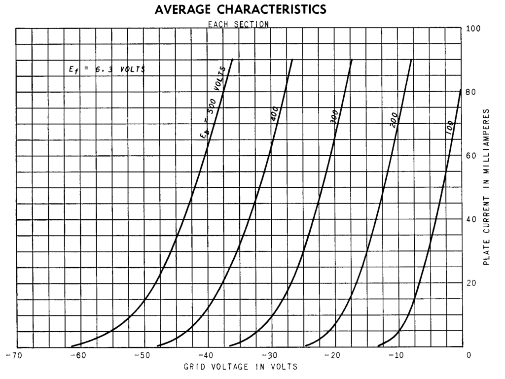
Page 4 contains the Average Plate Characteristics curve family used to fit the model. The curves were independently digitized from the original graph, producing a numerical dataset of plate current Ia as a function of plate voltage Va and grid voltage Vg.
Page 3, on the other hand, contains two different representations of the tube characteristics. These data were not used during fitting and were digitized separately to perform an independent validation of the model with the parameters already determined and frozen.
Important note: the data used in this work are not experimental measurements performed on a real tube sample. They are data independently digitized from the original General Electric datasheet.
The curves were digitized using Curve Digitizer, software developed by Giux-Lab to extract numerical data from graphs.
6BX7-GT SPICE model
The result of this work is a SPICE model of the 6BX7-GT, implemented as a three-terminal .SUBCKT: plate, grid, and cathode.
Download the 6BX7-GT SPICE model
The model describes the static characteristic: \[ I_a = f(V_a,V_g) \]
and is based on a global fit of the plate-characteristic family published by General Electric. The fitting dataset contains 440 points, distributed across grid-voltage curves from 0 V to −50 V.
Model parameters
| Parameter | Value |
|---|---|
| μ | 10.813884978151192 |
| Kp | 77.284607645620596 |
| Kvb | 654.33045589862036 |
| Kg1 | 485.64217355533503 |
| Ex | 1.3034825268711401 |
Fitting accuracy
| Metric | Value |
|---|---|
| RMSE | 1.069 mA |
| MAE | 0.851 mA |
| R² | 0.99659 |
The most important result, however, is not only the quality of the fit. The model was also tested using two datasets obtained from General Electric graphs not used during optimization.
Independent validation
| Dataset | Condition | N | RMSE | MAE | R² |
|---|---|---|---|---|---|
| GE page 3 — Ia(Va) | Within fitting domain | 214 | 1.242 mA | 0.975 mA | 0.99547 |
| GE page 3 — Ia(Vg) | Within fitting domain | 229 | 1.928 mA | 1.544 mA | 0.99005 |
These in-domain values are the most meaningful for evaluating the model under conditions covered by the data used to build it. Outside this region the model naturally continues to return a result, but it is then operating in extrapolation and the error can increase substantially.
The following sections define the model validity domain precisely and present the fitting, independent validations, and SPICE-translation verification separately.
Visual comparison with the datasheet curves
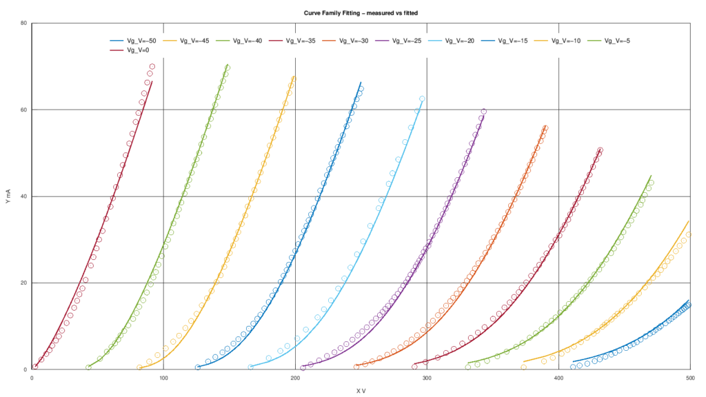
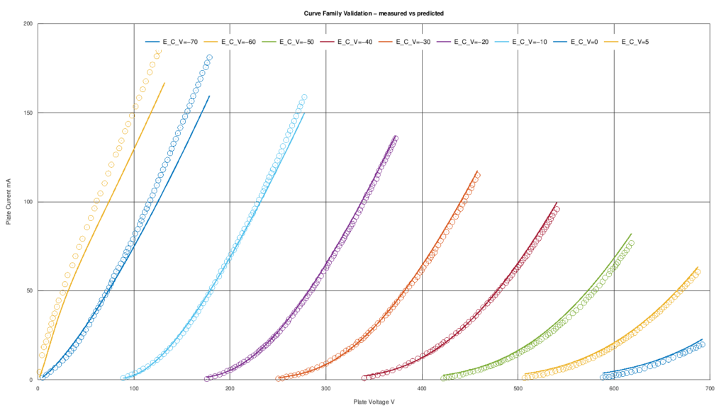
In addition to the numerical metrics, it is useful to inspect directly the comparison between the curve family digitized from the General Electric datasheet and the model obtained from the fit. The following graph shows the overlay between the digitized data and the curves generated by the model over the complete dataset used to construct the static characteristic.
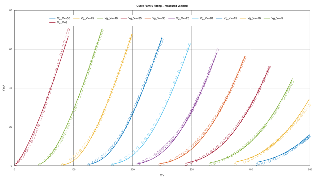
Download the high-resolution fitting plot
Note that this comparison concerns the data digitized from the datasheet used to fit the model. These are not experimental measurements performed on a real tube sample.
Model validity range
To use the 6BX7-GT SPICE model correctly, knowing its parameters is not enough: it is also necessary to know which region of the input-variable plane is supported by the data used for fitting.
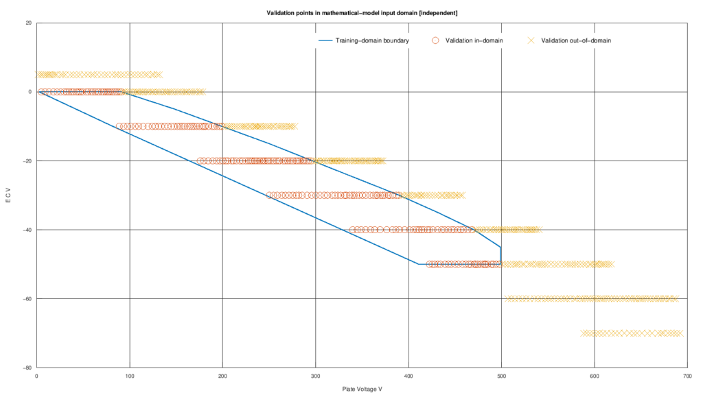
In this work, the model domain is not approximated by a simple rectangular interval defined by minimum and maximum values of Va and Vg. Instead, the fitting domain is represented by the convex hull of the points actually used for fitting in input space: \[ (V_a,V_g) \]
This choice makes it possible to distinguish rigorously between two different situations:
- in-domain interpolation, when the operating point lies inside the region covered by the fitting data;
- out-of-domain extrapolation, when the model is used outside that region.
It is important to note that domain classification uses only the model input variables, namely Va and Vg. The plate-current value Ia is not used to determine whether a point belongs to the fitting domain.
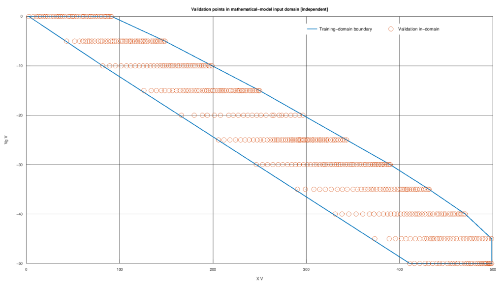
Download the high-resolution validity-domain plot
The distinction between points inside and outside this domain will be used in the following sections to interpret correctly the results of the independent validations obtained from the other General Electric datasheet graphs.
Independent model validation
The quality of the fit on the data used to build the model is not, by itself, sufficient to assess predictive performance. For this reason the model was subsequently tested using other data digitized from the same General Electric datasheet but not used during fitting.
The model parameters remained unchanged: no new optimization was performed during this phase. The new points therefore form an independent validation dataset with respect to the fitting data.
First validation: plate current versus plate voltage
The upper graph on page 3 of the GE datasheet shows plate current Ia as a function of plate voltage Va for several constant grid-voltage values:
\[ V_g = +5,\;0,\;-10,\;-20,\;-30,\;-40,\;-50,\;-60,\;-70\ \mathrm{V} \]In the original datasheet this voltage is labeled Ec; it is the control-grid voltage, not the cathode voltage.
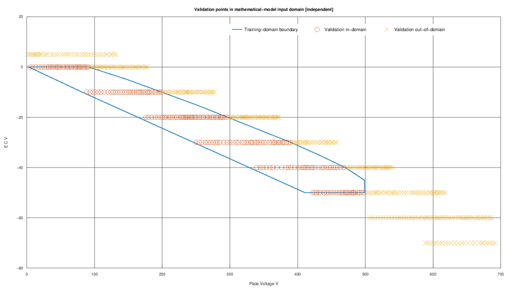
Which points are actually within the model domain?
Before interpreting the errors, the new points must be classified with respect to the domain defined by the fitting data. The following figure shows the position of the validation points in the Va–Vg plane.
Download the high-resolution validation-domain plot
This distinction is important because the page 3 datasheet graph extends well beyond the region covered by the curves used to build the model. In particular, this validation also includes grid voltages down to −70 V and plate voltages approaching 700 V.
Comparison with the SPICE model
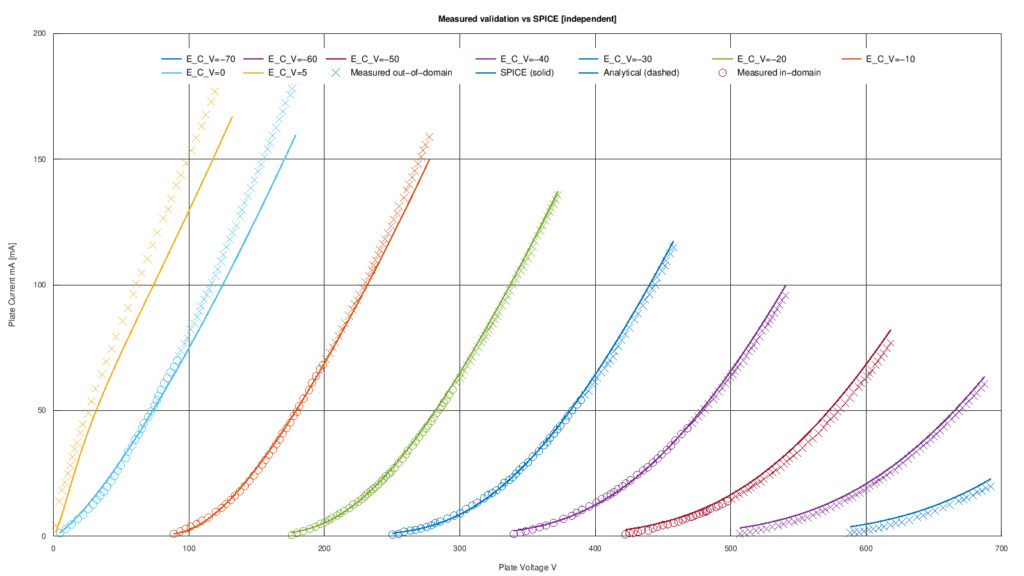
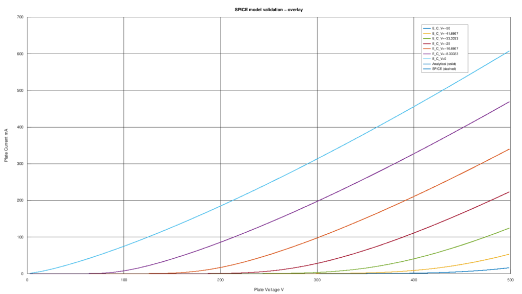
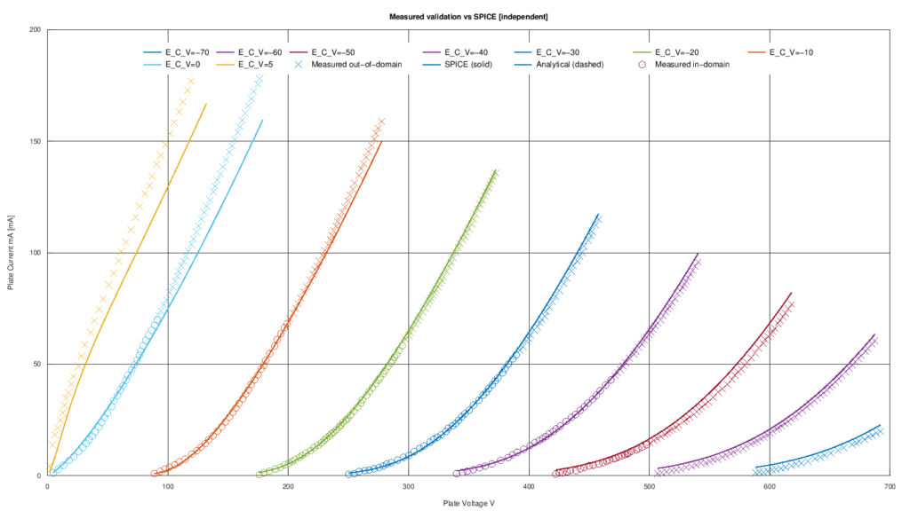
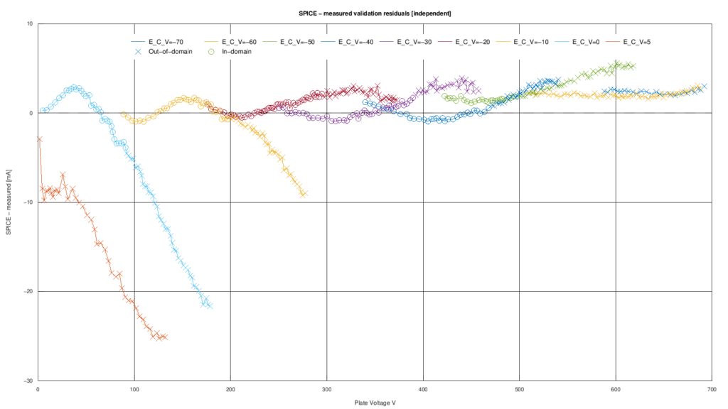
The following figure directly compares the data digitized from the GE datasheet with the SPICE-model response. Points inside and outside the domain are shown separately; both the SPICE solution and the solution of the mathematical model from which the SPICE model was derived are also plotted.
Download the high-resolution independent SPICE validation plot
The graphs generated by the software use the label measured. In this article it refers to data digitized from the General Electric datasheet, not experimental measurements performed on a real tube.
Quantitative results
| Region | N | RMSE | MAE | Maximum absolute error | R² |
|---|---|---|---|---|---|
| All points | 568 | 6.276 mA | 3.750 mA | 25.251 mA | 0.98102 |
| In-domain | 214 | 1.242 mA | 0.975 mA | 3.867 mA | 0.99547 |
| Out-of-domain | 354 | 7.890 mA | 5.428 mA | 25.251 mA | 0.97189 |
The most significant result is obtained on the 214 in-domain points: RMSE is 1.242 mA, with R² = 0.99547. These are data never used by the fitting process, but they fall within the region of Va–Vg space supported by the dataset used to build the model.
When points outside the training domain are considered, RMSE rises to 7.890 mA. The global value of 6.276 mA therefore mixes two physically and mathematically different situations: interpolation within the region covered by the data and extrapolation outside it.
For this reason, for practical use of the SPICE model, the in-domain metrics are more representative of its accuracy in the region for which it was actually built.
Second validation: plate current versus grid voltage
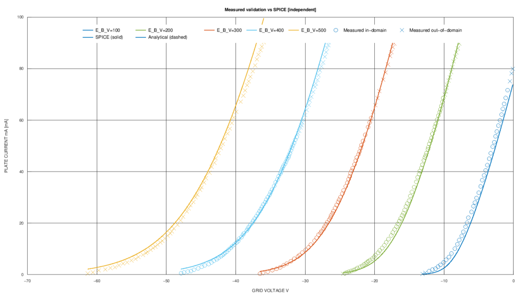
The second graph used for independent validation is the lower graph on page 3 of the General Electric datasheet. Here the representation is different: plate current Ia is plotted as a function of grid voltage Vg, while plate voltage is held constant. \[ V_a = 100,\;200,\;300,\;400,\;500\ \mathrm{V} \]
In the original datasheet the plate voltage is labeled Eb. These data were also digitized separately and were not used during fitting. The model parameters therefore remained exactly those determined previously.
This second test is particularly interesting because it observes the same static characteristic from a different direction. The model still describes the surface: \[ I_a = f(V_a,V_g) \]
but instead of traversing it by varying Va at constant grid voltage, it considers sections at constant Va while varying Vg.
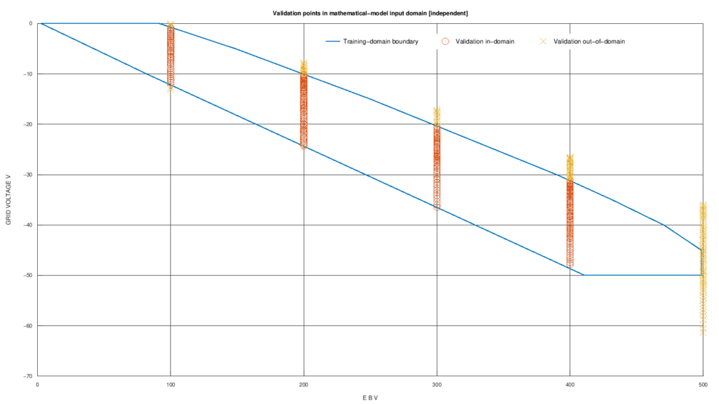
Distribution of points relative to the training domain
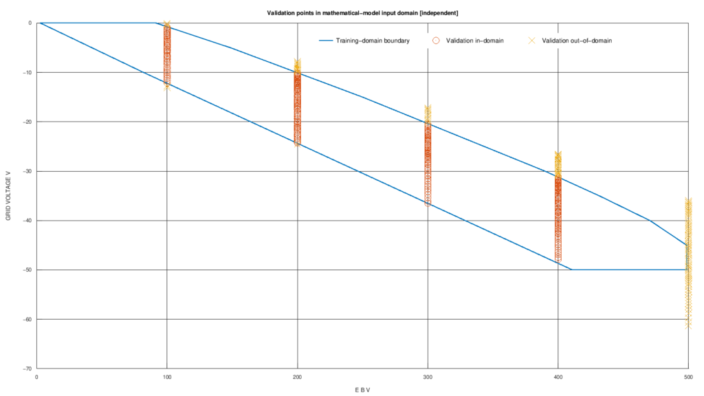
For this validation as well, the new points were classified against the same training domain defined by the data used for fitting.
Download the high-resolution domain plot for the second validation
In this representation, the five vertical columns correspond to plate voltages of 100, 200, 300, 400, and 500 V. For each of them, the grid-voltage intervals that fall inside or outside the domain covered by the fitting data can therefore be identified.
Comparison with the SPICE model
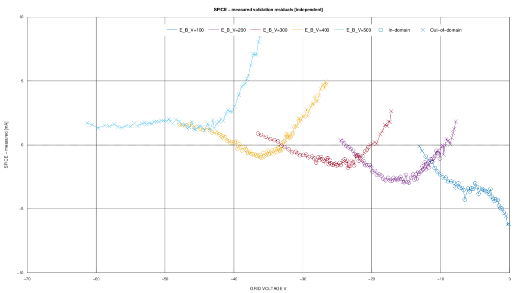
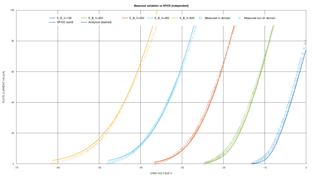
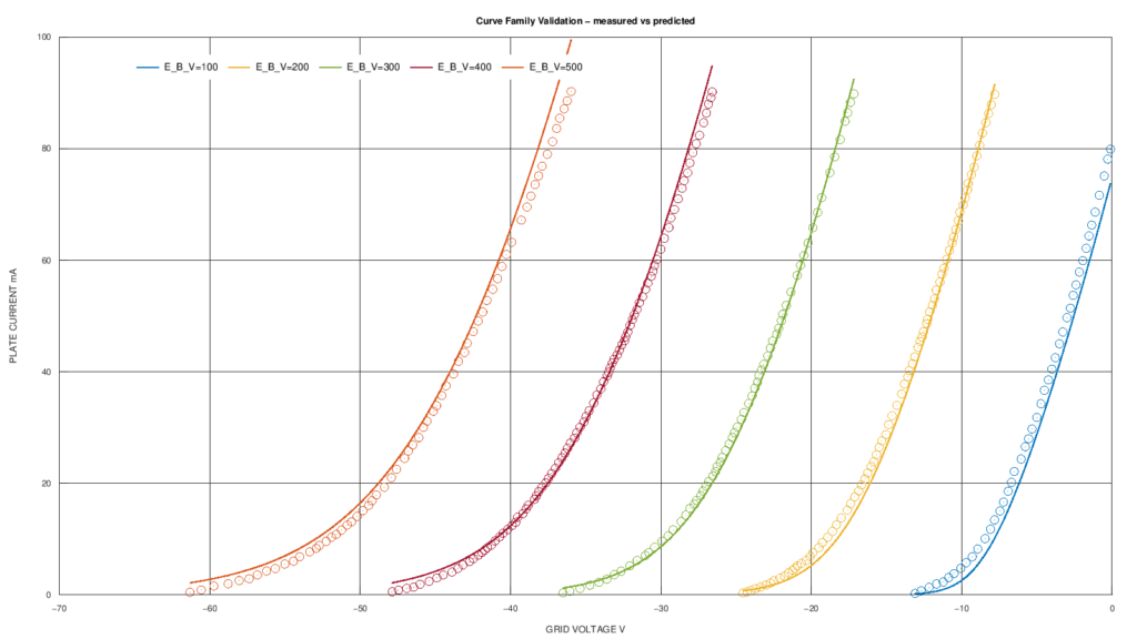
The following graph directly shows plate current as a function of grid voltage for the five plate voltages considered in the datasheet. The digitized GE data are compared with the SPICE model and with the corresponding analytical solution.
Download the high-resolution second SPICE validation plot
Quantitative results
| Region | N | RMSE | MAE | Maximum absolute error | R² |
|---|---|---|---|---|---|
| All points | 348 | 2.373 mA | 1.829 mA | 9.279 mA | 0.99194 |
| In-domain | 229 | 1.928 mA | 1.544 mA | 5.295 mA | 0.99005 |
| Out-of-domain | 119 | 3.051 mA | 2.379 mA | 9.279 mA | 0.98992 |
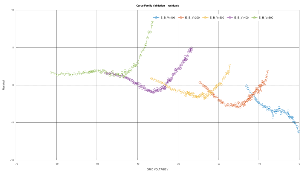
This second validation also confirms good agreement within the region covered by the fitting data. On the 229 in-domain points, RMSE is 1.928 mA, while the maximum absolute error is 5.295 mA.
When the model is used outside the training domain, RMSE rises to 3.051 mA and the maximum absolute error reaches 9.279 mA. Here too, separating interpolation from extrapolation makes it possible to interpret model performance more meaningfully than a single global metric.
Verification of the SPICE translation
Validation against the datasheet measures how well the model represents the characteristics published by General Electric. There is, however, a second and distinct question: whether translating the mathematical model into a SPICE .SUBCKT introduces any additional error.
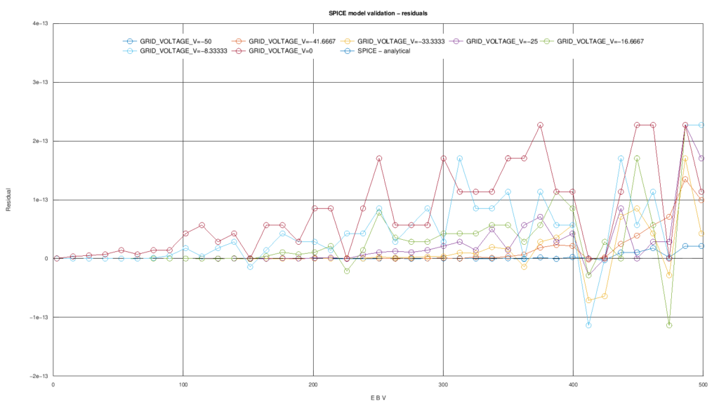
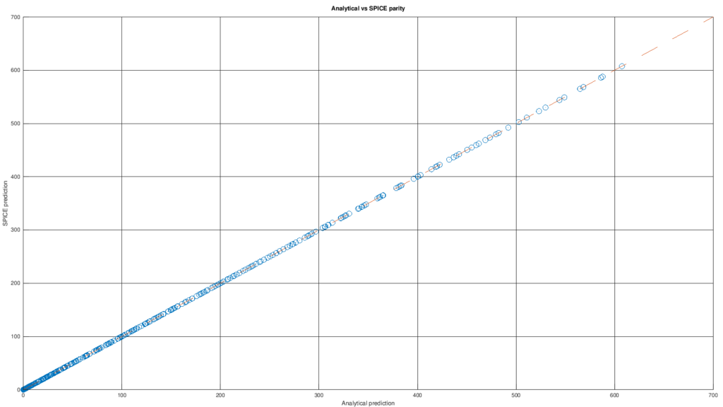
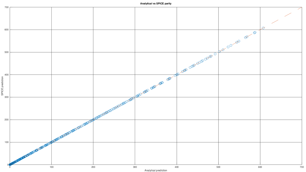
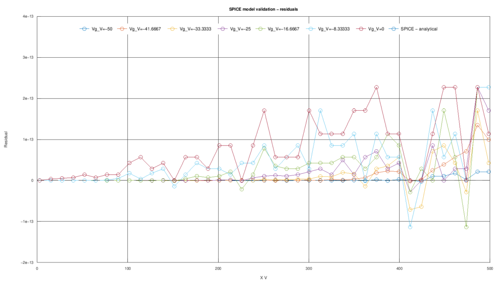
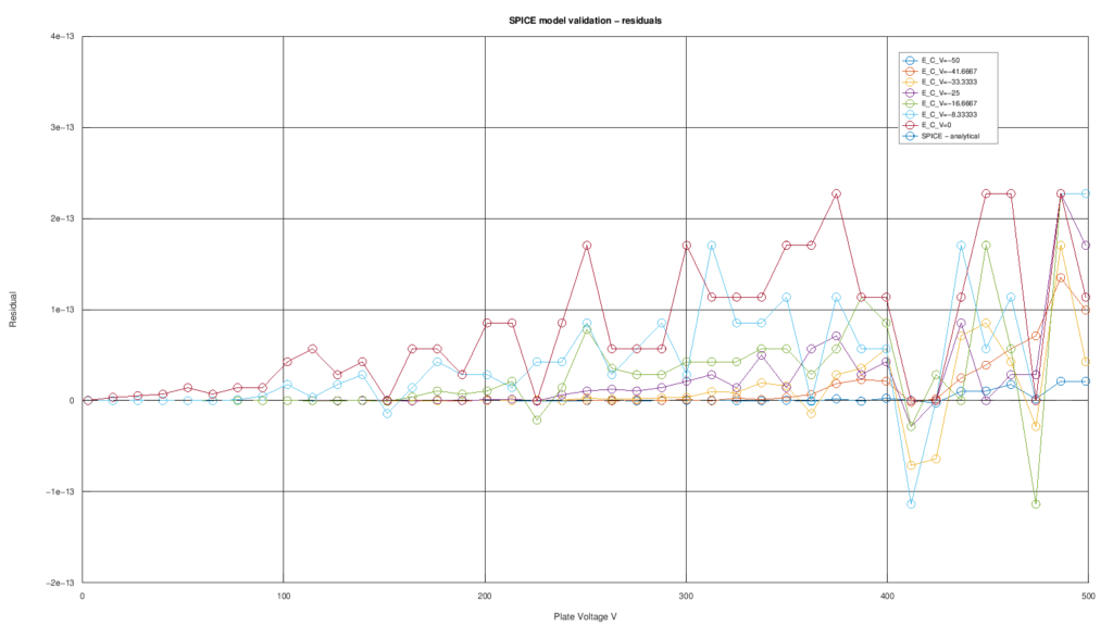
For this reason, the SPICE model was compared directly with the mathematical function from which it was derived, automatically using two sweep types and a total of 574 operating points.
| Metric | SPICE vs mathematical model |
|---|---|
| N | 574 |
| RMSE | 5.96 × 10⁻¹⁴ mA |
| MAE | 3.19 × 10⁻¹⁴ mA |
| Maximum absolute error | 2.84 × 10⁻¹³ mA |
| R² | 1 |
| Result | PASS |
The differences are on the order of numerical error. The SPICE representation can therefore be considered numerically equivalent to the mathematical function used for fitting.
This verification does not prove that the physical model is perfect; it demonstrates something different and equally important. The errors observed when comparing against the data digitized from the GE datasheet belong to the mathematical model and its ability to represent the tube, and are not introduced by the SPICE conversion.
Model limitations and correct use
The SPICE model presented in this article represents only the static plate characteristic of the 6BX7-GT: \[ I_a = f(V_a,V_g) \]
It is therefore suitable for simulations in which the relevant quantity is the relationship between plate voltage, grid voltage, and plate current under the conditions described and validated in the previous sections.
The model does not include:
- grid current;
- interelectrode capacitances;
- filament and heater behavior;
- thermal effects;
- secondary emission;
- other dynamic phenomena not included in the static law used for fitting.
Consequently, the .SUBCKT should not be interpreted as a
complete model of all the physical phenomena of the 6BX7-GT. It is a
quantitative representation of its static plate characteristic,
built from General Electric data and independently verified
against other curves from the same datasheet.
Use inside and outside the fitting domain
For quantitative use of the model, it is also necessary to consider the position of the operating point relative to the training domain shown in the previous sections.
A point inside the domain is an in-domain interpolation condition: the model is being used in a region directly supported by the data used to determine its parameters. The two independent validations produced RMSE values in this region of 1.242 mA and 1.928 mA, respectively.
A point outside the domain is instead an out-of-domain extrapolation condition. The SPICE model continues to return a solution, but that solution is not directly supported by the fitting dataset and should therefore be used with greater caution.
To determine whether a given combination of Va and Vg belongs to the model domain, it is not sufficient to check the minimum and maximum values of the two voltages separately: the training domain is defined by the convex hull of the points actually used for fitting. The Va–Vg map shown above is therefore the correct reference.
From the datasheet to the mathematical model
The model is built from the Average Plate Characteristics family shown on page 4 of the General Electric 6BX7-GT datasheet.
Eleven plate characteristics were independently digitized, corresponding to the following grid voltages: \[ V_g = 0,\;-5,\;-10,\;-15,\;-20,\;-25,\;-30,\;-35,\;-40,\;-45,\;-50\ \mathrm{V} \]
The final dataset contains 440 points. Each point associates a plate voltage Va, a grid voltage Vg, and the corresponding plate current Ia obtained from the original graph: \[ I_a = f(V_a,V_g) \]
These data form the dataset used to determine the model parameters simultaneously across the entire curve family. No separate fit was performed for each characteristic.
The Koren model
To represent the 6BX7-GT characteristics mathematically, a formulation based on the Koren triode model was used.
The theory of the model, the meaning of its parameters, and its main limitations are discussed separately in the article Koren model for triodes: theory and limitations . Here we focus instead on its concrete application to the 6BX7-GT and on determining the parameters from the General Electric data.
The formulation used for fitting
The 6BX7-GT fitting used the
triode.koren_v1 implementation. The model takes
plate voltage Va and grid-to-cathode voltage
Vg as input variables and calculates plate current
Ia.
The implemented formulation can first be written by introducing: \[ D = \sqrt{\max\!\left(K_{vb}+V_a^2,\varepsilon\right)} \] \[ z = K_p\left( \frac{1}{\mu} + \frac{V_g}{D} \right) \]
The exponential term is evaluated using a numerically stable form of the softplus function: \[ S(z)=\max(z,0)+\ln\!\left(1+\exp(-|z|)\right) \]
which is mathematically equivalent to: \[ S(z)=\ln\!\left(1+\exp(z)\right) \]
but avoids numerical problems when z has a large magnitude. The following quantity is then calculated: \[ E_1 = \max\!\left[ \frac{V_a}{K_p}S(z), 0 \right] \]
and finally the plate current, expressed in milliamperes: \[ I_a\,[\mathrm{mA}] = \frac{2000}{K_{g1}}E_1^{E_x} \]
The factor 2000 comes from combining Koren’s 1 + sign(E1) factor, which equals 2 in the positive-current region, with the conversion from current in amperes to current expressed in milliamperes.
This is the actual equation used to determine the five parameters μ, Kp, Kvb, Kg1, and Ex of the 6BX7-GT. It is also the same static law later translated into the SPICE model.
Global fitting of the curve family
The five model parameters were not determined separately for each plate characteristic. A global fit was performed using all 440 points digitized from the eleven General Electric curves simultaneously.
The general procedure used to fit a Koren model to the characteristic curves of a triode is described in detail in the article From datasheet to SPICE model: Koren fitting of the 6BX7-GT . Here only the data and results specific to the 6BX7-GT model used in this work are reported.
For each point in the dataset, the model calculates a predicted plate current, which is compared with the digitized value Ia. The residual for each individual point can be written as: \[ r_i = \hat{I}_{a,i} – I_{a,i} \]
The optimization determines a single parameter set: \[ \theta = \left( \mu,\; K_p,\; K_{vb},\; K_{g1},\; E_x \right) \]
valid for the entire family of characteristics.
Final parameters
| Parameter | Value |
|---|---|
| μ | 10.813884978151192 |
| Kp | 77.284607645620596 |
| Kvb | 654.33045589862036 |
| Kg1 | 485.64217355533503 |
| Ex | 1.3034825268711401 |
Once fitting was complete, this parameter set was frozen and used without further modification both for the independent validations and for subsequent SPICE-model generation.
Fitting quality
| Metric | Value |
|---|---|
| RSS | 502.6329 |
| RMSE | 1.0688 mA |
| MAE | 0.8505 mA |
| R² | 0.99659 |
These metrics describe how well the model reproduces the data used to determine its parameters. By themselves, however, they do not constitute an independent test of predictive performance; for that reason, the two validations on the page 3 General Electric datasheet graphs were performed separately, as shown in the previous sections.
From the mathematical model to the SPICE model
Once the five parameters had been determined and frozen, the same static law used during fitting was translated into a three-terminal SPICE model: plate, grid, and cathode.
The distributed model is a standard .SUBCKT and directly contains
the parameters obtained from fitting:
.SUBCKT GXTXT_MODEL plate grid cathode

.param mu=10.813884978151192 Kp=77.284607645620596
       + Kvb=654.33045589862036 Kg1=485.64217355533503
       + Ex=1.3034825268711401
The voltages used by the law are referenced to the cathode: \[ V_a = V(\mathrm{plate},\mathrm{cathode}) \] \[ V_g = V(\mathrm{grid},\mathrm{cathode}) \]
Plate current is generated by a behavioral source
BPLATE connected between plate and cathode. In the actual SPICE file,
the structure is:
BPLATE plate cathode I={ ... }

.ENDS GXTXT_MODEL
The expression contained in BPLATE directly implements the same
mathematical law used for fitting. No second model or additional SPICE-specific
approximation is introduced: the function is simply expressed
using the simulator’s behavioral-source syntax.
The SPICE formulation also preserves the numerical safeguards present in the mathematical implementation, including the stable evaluation of the logarithmic-exponential term and protections against numerically problematic values.
The correctness of the translation was verified by automatically comparing
the .SUBCKT with the original mathematical model over
574 operating points. The resulting RMSE is
5.96 × 10⁻¹⁴ mA, with
R² = 1: the differences are therefore essentially limited
to numerical precision.
Real-world test of the model with ngspice
To verify the practical use of the spice_model.lib file as well,
the model was run directly with ngspice on the server,
using a simple testbench external to the fitting and validation system.
The tube model file is included normally:
.include "spice_model.lib"The subcircuit is then instantiated by connecting plate, grid, and cathode:
X1 plate grid 0 GXTXT_MODELThe complete testbench used is:
* 6BX7-GT - real test of the published model

.include "spice_model.lib"

* Plate supply
VPLATE nsource 0 0

* 0 V source used to measure Ia with positive sign
VMEAS nsource plate 0

* Grid-to-cathode voltage
VGRID grid 0 0

* 6BX7-GT model
X1 plate grid 0 GXTXT_MODEL

* Va: 0 -> 500 V, 5 V step
* Vg: 0 -> -50 V, -5 V step
.dc VPLATE 0 500 5 VGRID 0 -50 -5

.control
run
plot i(VMEAS)
.endc

.end
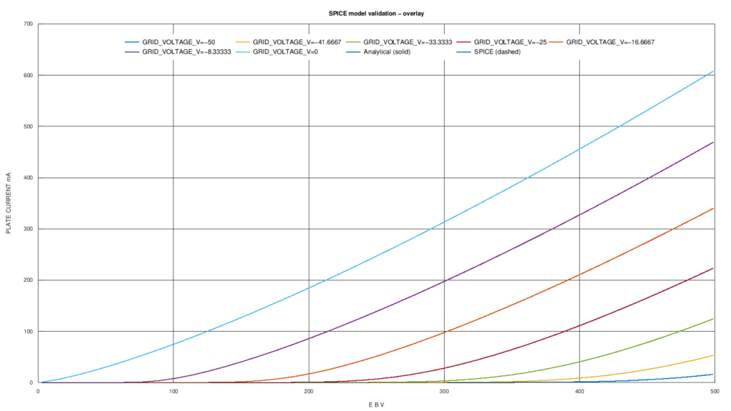
The simulation sweeps plate voltage from 0 to 500 V for eleven grid-voltage values between 0 and −50 V, thus reproducing the same family of conditions used to characterize the model.
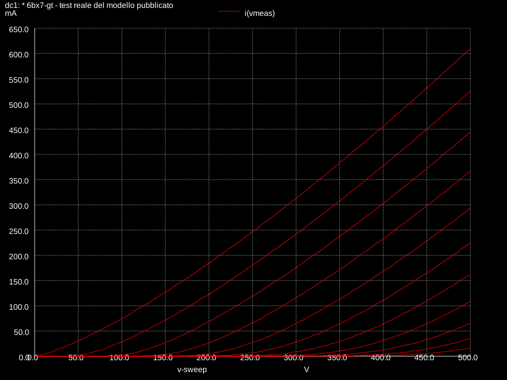
Open the ngspice simulation plot in vector format
This test uses the .lib file intended for distribution directly
and shows that the model can be included and simulated with ngspice
without any additional transformation.
Conclusions
The 6BX7-GT SPICE model presented in this article comes from a global fit of 440 points digitized from the plate characteristics published by General Electric.
Verification was not limited to the data used to determine the parameters. The model was compared with two additional sets of curves from the same datasheet, digitized separately and never used during optimization. This made it possible to evaluate separately the behavior in interpolation inside the training domain and in extrapolation outside it.
The subsequent SPICE translation was verified separately against the
original mathematical model. Over 574 operating points, the error between the
two representations was on the order of 10−13 mA, showing that the
conversion to the .SUBCKT does not introduce significant error with respect
to the mathematical function from which it is derived.
Finally, the distributed spice_model.lib file was
used directly in a real ngspice simulation, reproducing the
family of plate characteristics for grid voltages from
0 to −50 V.
The result is therefore a SPICE model accompanied not only by its parameters and simulation file, but also by an explicit definition of its validation range and limitations. It remains a model of the static plate characteristic: capacitances, grid current, thermal effects, and other dynamic phenomena would require further extensions.
Technical gallery and validation plots
The following galleries collect the plots used while building, verifying, and validating the 6BX7-GT model. They include the original General Electric datasheet graphs used for digitization, fitting results, independent validations, and comparisons between the mathematical model and the SPICE implementation.
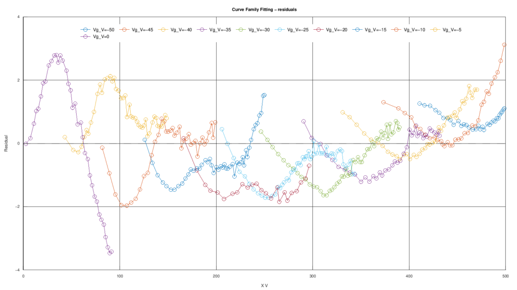
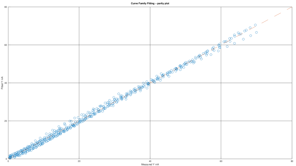
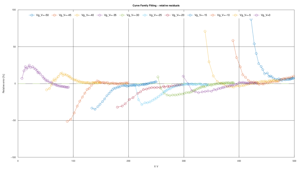
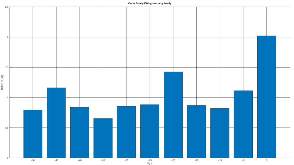
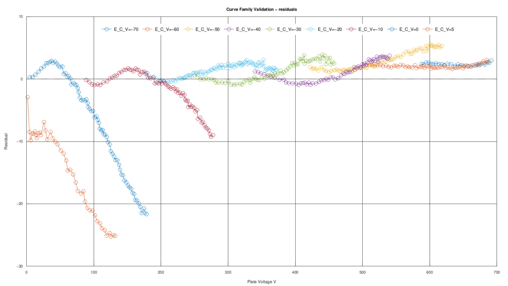
This gallery documents the process used to build the 6BX7-GT mathematical model from the General Electric datasheet curves. It begins with the original page 4 graph from which the fitting data were digitized, followed by comparisons between digitized data and the model, residual analyses, and summary error indicators.
This gallery collects the plots related to verification of the 6BX7-GT SPICE model and its validation on data independent of the fitting process. It includes both the direct comparison between the mathematical model and the SPICE subcircuit and validation plots against digitized General Electric datasheet curves not used during optimization.
The plots generated by the software may use the label measured: in this context it refers to data digitized from the GE datasheet, not experimental measurements performed on a real tube.
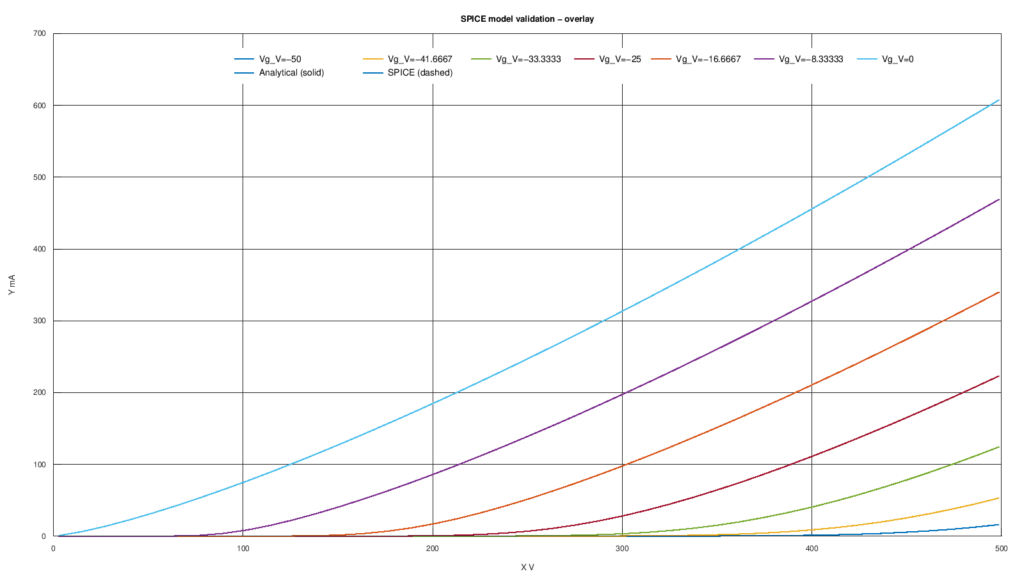
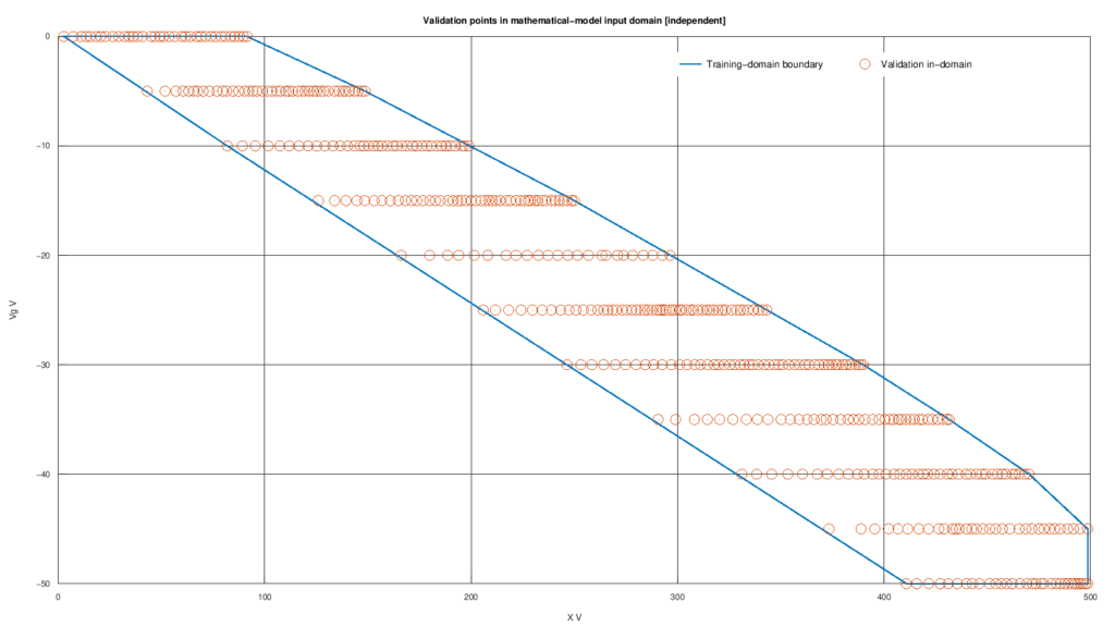
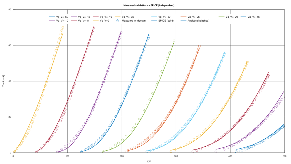
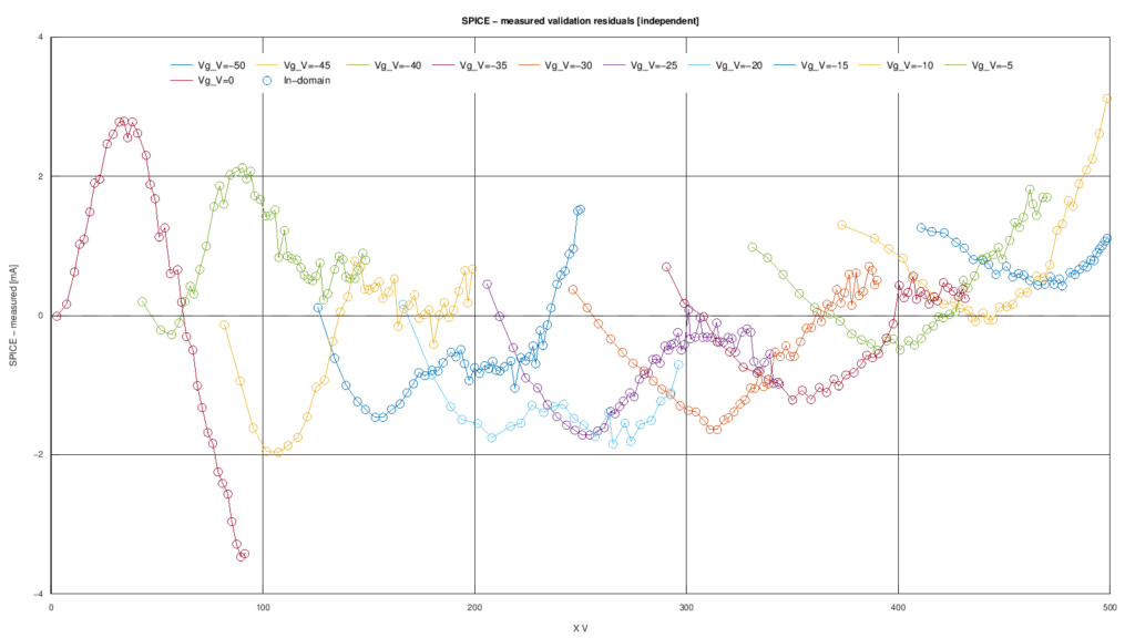
This gallery collects the main diagnostic plots from the first independent validation of the 6BX7-GT model, performed using the upper graph on page 3 of the General Electric datasheet, which was not used during fitting. The first image shows the original graph that was digitized; the following figures compare the data extracted from the datasheet with the model predictions and show the error distribution.
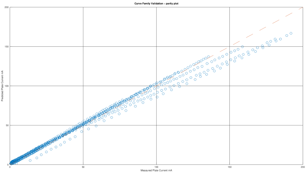
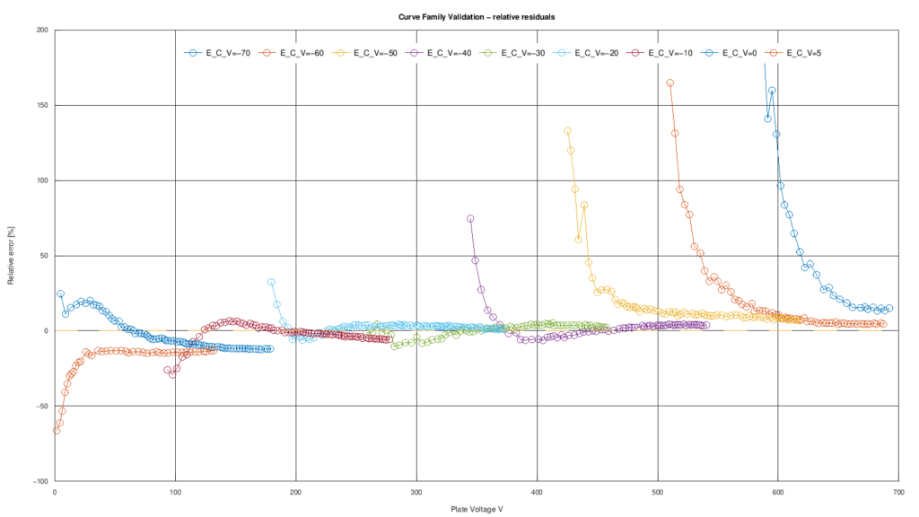
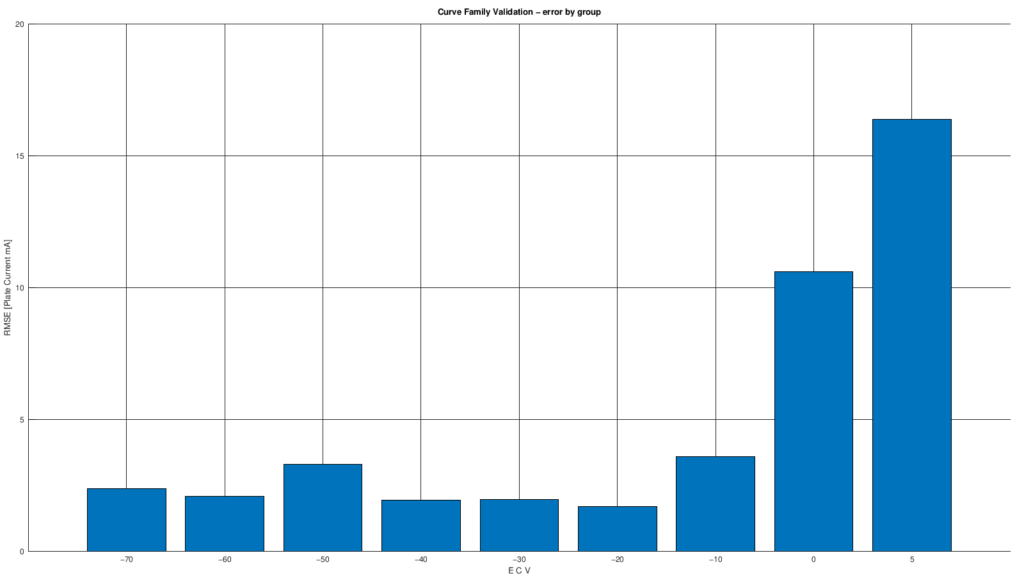
This gallery collects the plots related to verification of the 6BX7-GT SPICE subcircuit and its validation on the first independent dataset, obtained from the upper graph on page 3 of the General Electric datasheet. It includes both the comparison between the mathematical and SPICE implementations and the comparison between digitized datasheet data and SPICE-model predictions.
The plots may use the label measured: in this context it refers to data digitized from the GE datasheet, not experimental measurements performed on a real tube.
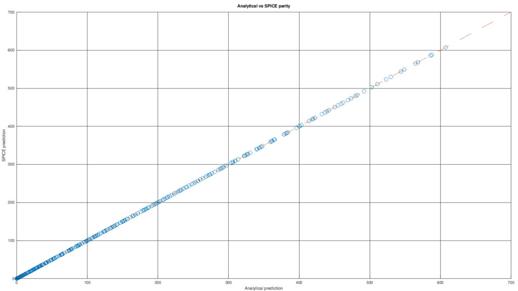
This gallery collects the diagnostic plots from the second independent validation of the 6BX7-GT model, performed using the lower graph on page 3 of the General Electric datasheet. In this case, plate current is plotted as a function of grid voltage at constant plate voltages of 100, 200, 300, 400, and 500 V.
The first image shows the original graph used for digitization; the following figures compare the data extracted from the datasheet with model predictions and show the error distribution. This dataset is also independent of the one used for fitting.
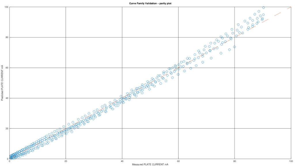
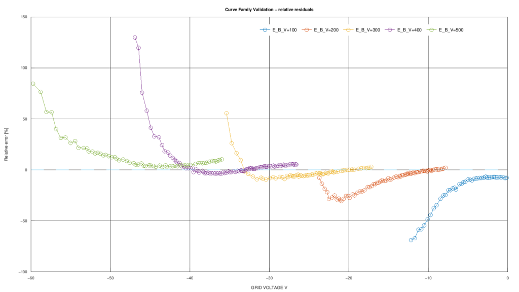
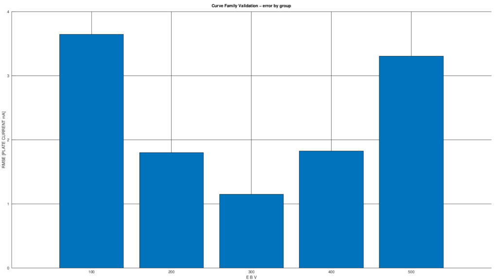
This gallery collects the validation plots for the SPICE version of the 6BX7-GT model. In the first images, the subcircuit is compared with an independent dataset to show how the exported model behaves on digitized points both inside and outside the fitting domain. The final images instead show the direct comparison between the analytical and SPICE implementations, confirming that the ngspice testbench correctly reproduces the mathematical model.