

Lesson 14 – Differential Equations: Chemical Kinetics with GNU Octave and GX-TXT
A chemical reaction rate can be expressed as a derivative. When several chemical species are transformed simultaneously, we obtain a system of ordinary differential equations (ODEs). In this lesson, we build a complete kinetic model, solve it with GNU Octave, verify conservation laws, and publish the results as GX-TXT Datasets and scientific plots.
Version note: in the GX-TXT P008 release used for these tests, the framework’s public ODE functionality had a callback transport issue. The published scripts therefore solve the system using GNU Octave ode45. Later in this article, we will describe the corresponding GX-TXT API, distinguishing its documented contract from the experimental results actually verified here.
Learning objectives
By the end of this lesson, we will be able to represent an ODE system with a state vector, define an anonymous Octave function, integrate with ode45, set numerical tolerances, compare a numerical solution with an analytical one, apply a physical consistency check, and publish reproducible results through GX-TXT’s public APIs. We will also revisit the debugger introduced in previous lessons.
What we already know and what we will learn next
In the first thirteen lessons, we learned to write Octave scripts, work with vectors and matrices, organize GX-TXT Datasets, publish persistent plots, and check for errors. In Lesson 04, we even simulated cooling using Euler’s method; in Lesson 11, we calculated derivatives and integrals from existing data. Our next step is different: we start with a law describing a derivative and seek the unknown time evolution.
Lesson 12 provided the matrix language needed to represent several coupled quantities; Lesson 13 showed how the same phenomenon can be studied in different representations, such as time and frequency. Here we introduce an initial-value problem, a dynamical system, and an adaptive numerical solver. The GX-TXT Dataset, publication, and plotting APIs are tools we have already encountered; we use them again to show how an ODE simulation can be made reproducible.
| Previous knowledge | New in Lesson 14 |
|---|---|
| Lesson 04: Euler integration for cooling | Adaptive integration of three coupled equations with ode45 |
| Lesson 11: differentiation/integration of sampled data | Reconstructing a trajectory from its differential law |
| Lesson 12: matrix algebra | State vectors and production/consumption contributions |
| Lesson 13: comparing methods and reconstruction | Physical validation using mass balance and the analytical solution |
Experiment: two consecutive reactions
Consider two irreversible first-order transformations:
\[ A \xrightarrow{k_1} B \xrightarrow{k_2} C \]
The reaction rates are \(v_1=k_1[A]\) and \(v_2=k_2[B]\). Therefore:
\[ \frac{d[A]}{dt}=-k_1[A],\qquad \frac{d[B]}{dt}=k_1[A]-k_2[B],\qquad \frac{d[C]}{dt}=k_2[B]. \]
The first term makes A decrease; B is produced by the first reaction and consumed by the second, while C accumulates. The minus sign in the B consumption term is not a syntactic detail: it follows from the physical reaction mechanism.
We assume \(k_1=0.240\,\mathrm{min}^{-1}\), \(k_2=0.075\,\mathrm{min}^{-1}\) and the initial conditions \([A](0)=2.000\,\mathrm{mmol/L}\), \([B](0)=[C](0)=0\). We will study the interval from 0 to 40 minutes, sampled every 0.5 minutes: 81 time points.
What is conserved? Because A, B, and C represent the same amount of substance transferred among three forms, with no inflow or loss and with unit stoichiometry,
\[ [A](t)+[B](t)+[C](t)=[A](0)=2.000\,\mathrm{mmol/L}. \]
This equality provides a check independent of the numerical algorithm.
From reaction rates to equations
A first-order reaction has a rate proportional to the reactant concentration. In our case, the A → B transformation has rate \(v_1=k_1 A\), while B → C has rate \(v_2=k_2 B\). A disappears only in the first reaction; B is formed in the first and disappears in the second; C is formed only in the second.
We can express these rules as a stoichiometric matrix, drawing on what we learned in linear algebra:
\[ \frac{d\mathbf{y}}{dt}=\underbrace{\begin{bmatrix}-1&0\\1&-1\\0&1\end{bmatrix}}_{S}\underbrace{\begin{bmatrix}k_1 A\\k_2 B\end{bmatrix}}_{\mathbf{v}}. \]
The sum of the entries in each column of \(S\) is zero: each transformation removes matter from one species and adds it to another. Adding the three equations therefore gives \(\frac{d}{dt}(A+B+C)=0\). This is an invariant of the model, not an accidental result of the software. The balance holds because we assumed unit stoichiometry and a closed system.
The rate constants have units of \(\mathrm{min}^{-1}\), concentrations have units of \(\mathrm{mmol/L}\), and their derivatives have units of \(\mathrm{mmol\,L^{-1}\,min^{-1}}\). Dimensional analysis provides an initial check of the model even before running the code.
The state vector in GNU Octave
To solve a coupled system, we collect the concentrations into a column vector:
\[ \mathbf{y}(t)=\begin{bmatrix}A(t)\\B(t)\\C(t)\end{bmatrix},\qquad \frac{d\mathbf{y}}{dt}=f(t,\mathbf{y}). \]
In GNU Octave, we write:
k1 = 0.24;
k2 = 0.075;
initial_state = [2; 0; 0];
rhs = @(t,y) [-k1*y(1); k1*y(1)-k2*y(2); k2*y(2)];
The semicolons inside square brackets create a column vector. The expressions y(1), y(2), and y(3) access the three concentrations, respectively. The syntax @(t,y) creates an anonymous function, that is, a function that can be passed as an argument to another function; here it depends on time and on the state vector. Even though our reaction rates do not depend explicitly on time, the solver’s required signature includes it.
Why the solver needs an anonymous function
The expression rhs = @(t,y) ... does not immediately compute all the concentrations: it defines a function handle that Octave can call repeatedly with a trial time and state. The constants k1 and k2 belong to the environment in which the function is defined; Octave retains the necessary values. The name rhs stands for right-hand side of the differential equation.
We do not put the analytical solution into this function: we describe only the local rate of change. The task of ode45 is to reconstruct the trajectory from that rule and the initial state.
Solving the system with ode45
GNU Octave’s ode45 function uses an adaptive Runge–Kutta method for non-stiff problems. It does not simply apply a fixed 0.5-minute step: it adjusts the internal step size to satisfy the requested tolerances and returns the solution at the specified times.
time_min = (0:0.5:40)';
options = odeset('RelTol',1e-8, ...
                 'AbsTol',1e-10, ...
                 'MaxStep',0.25);
[solved_time, state] = ode45(rhs,time_min,initial_state,options);
odeset prepares the solver options. RelTol controls relative error, AbsTol controls absolute error, and MaxStep limits the maximum internal step. These are numerical settings, not experimental uncertainties. The state result has one row for each time point and three columns: A, B, and C. A solver completing without errors is not enough: we must also check that the result is physically plausible.
Internal steps, output times, and tolerances
It is important to distinguish three levels. The vector time_min = (0:0.5:40)' specifies the 81 times at which we want results; it does not force the solver to integrate using fixed 0.5-minute steps. The Runge–Kutta 4(5) method used by ode45 estimates local error and chooses smaller or larger internal steps. The MaxStep = 0.25 option sets an upper limit on internal steps, not on the spacing between output rows.
| Option | Educational meaning |
|---|---|
RelTol = 1e-8 | Relative target for local error control |
AbsTol = 1e-10 | Absolute scale below which a small component cannot be assessed using relative error alone |
MaxStep = 0.25 | Maximum allowed internal step (in the time unit: minutes) |
These settings affect accuracy and computational cost, but they do not represent uncertainty in measured concentrations. ode45 is appropriate here because the problem is non-stiff; for kinetics involving very different timescales, it may be worth considering a stiff solver such as ode15s, after checking its availability and behavior in the installed version of Octave.
The returned state matrix has 81 rows and three columns. state(:,1) is the trajectory of A, state(:,2) that of B, and state(:,3) that of C. The apostrophe after the time expression creates a column vector; it should not be mistaken for differentiation with respect to time.
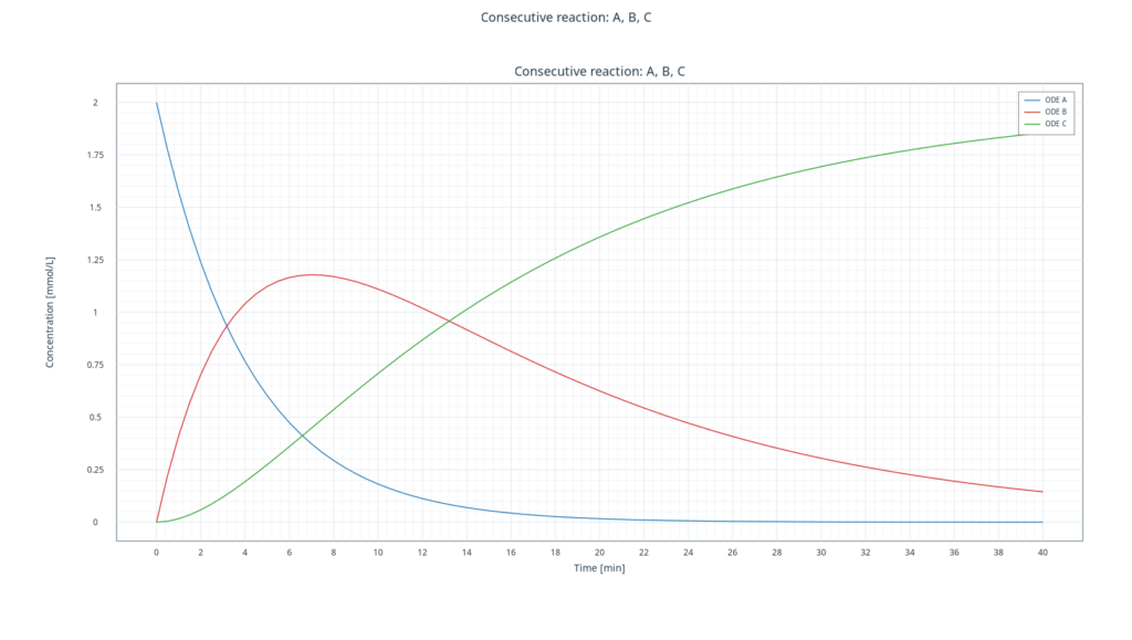
In the plot, A decreases, C increases, and B exhibits an intermediate maximum. This is the expected behavior of a species produced by one reaction and consumed by another.
An analytical solution as a reference
For \(k_1\ne k_2\), the system has a closed-form solution:
\[ A(t)=A_0 e^{-k_1 t}, \]
\[ B(t)=A_0\frac{k_1}{k_2-k_1}\left(e^{-k_1 t}-e^{-k_2 t}\right), \]
\[ C(t)=A_0-A(t)-B(t). \]
In the first lesson script, we generate three reference Datasets from these formulas. In the third script, we read them back through their Variable IDs and compare the ode45 solution with the formulas, sample by sample.
The time at which B reaches its maximum is found by imposing \(\frac{dB}{dt}=0\):
\[ t_{\max,B}=\frac{\ln(k_1/k_2)}{k_1-k_2}. \]
With our chosen parameters, this time is approximately 7.05 minutes. The peak concentration is approximately 1.18 mmol/L. The peak identified among discrete samples may occur at a slightly different time: the plot is sampled every half minute, whereas the analytical extremum lies between two samples.
Why B reaches a maximum
Initially, B is absent, so the production term \(k_1 A\) dominates. Later, A becomes depleted and the consumption term \(k_2 B\) takes over. At the maximum, the two rates are equal: \(k_1 A=k_2 B\). This compares instantaneous rates, not total quantities.
The analytical formula gives approximately 7.049399 min and 1.178736 mmol/L. On the half-minute output grid, the observed maximum instead occurs near 7.0 min. This difference in peak position does not prove an integration error: it results from the discretization used to read the curve and must be distinguished from the solver’s error.
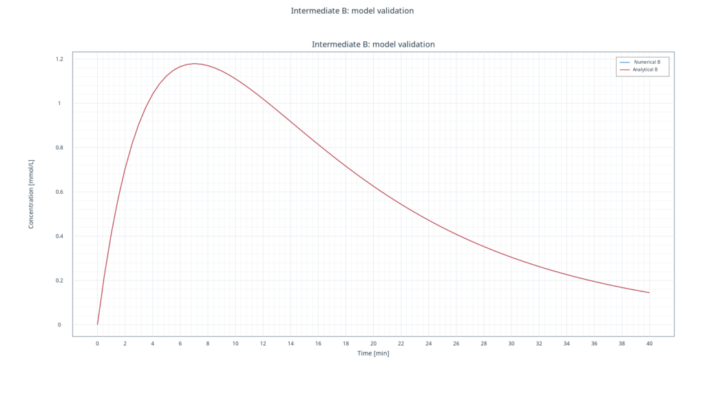
For a quantitative check, we use the maximum-error norm: we calculate max(abs(state-reference)) across all three species and all time points. In the lesson run, the discrepancy is on the order of \(10^{-10}\,\mathrm{mmol/L}\), well below the teaching threshold of \(10^{-5}\,\mathrm{mmol/L}\).
Numerical validation and physical validation
The first check measures the numerical solution’s error against an independent analytical solution. The second measures the residual of a physical law: both are needed. In the corrected code, we construct the matrix model_difference = state - reference and flatten it with model_difference(:) to find a single maximum across all 81 × 3 values:
model_difference = state - reference;
maximum_reference_error = max(abs(model_difference(:)));
conservation_error = sum(state, 2) - initial_state(1);
maximum_conservation_error = max(abs(conservation_error));
Be careful: applying max(abs(state-reference)) directly to a matrix produces maxima by column, not automatically a single scalar. The (:) suffix is therefore an important step, not merely a syntactic embellishment.
| Check | Lesson result | Interpretation |
|---|---|---|
| Maximum deviation from analytical solution | ≈ 2.98 × 10⁻¹⁰ mmol/L | Numerical integration consistent with the reference |
| Maximum conservation residual | ≈ 8.88 × 10⁻¹⁶ mmol/L | Total concentration constant within rounding precision |
| Returned samples | 81 | 0–40 min, output interval 0.5 min |
The conservation residual must not be interpreted as experimentally measured missing mass: values close to machine precision reflect floating-point arithmetic.
Debugging: a reaction that creates matter from nothing
The second script contains an error deliberately introduced for us to find:
wrong_rhs = @(t,y) [-k1*y(1); ...
                    k1*y(1)+k2*y(2); ...
                    k2*y(2)];
In the second component, we wrote +k2*y(2) instead of -k2*y(2). Species B is incorrectly produced rather than consumed in the second step, while C continues to form. The calculation may return finite values and a smooth curve, but the model is wrong.
We calculate the total at each time point:
total = sum(state,2);
maximum_conservation_error = ...
    max(abs(total-initial_state(1)));
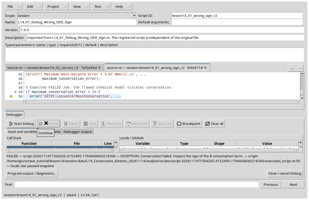
sum(state,2) sums the three concentrations across each row. If the total increases instead of remaining constant, mass conservation is violated. The script then raises an explicit error with identifier GXTXT:Lesson14:MassConservation, marking the Job as failed for a verifiable scientific reason.
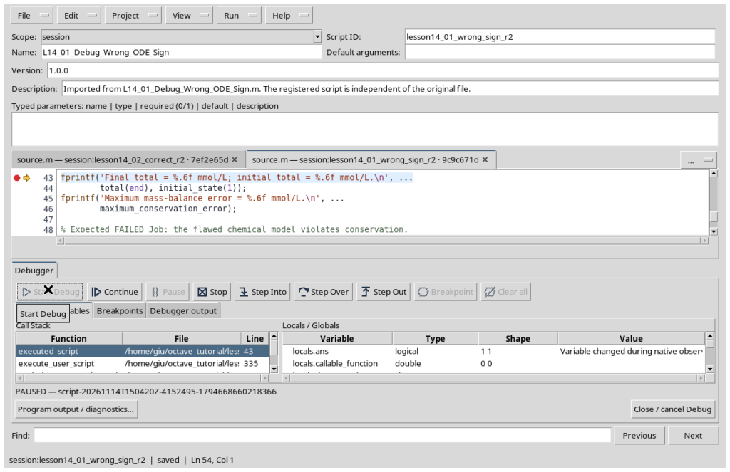
We start the debugger with Run → Debug Session script, place a breakpoint before the mass-balance result is printed, and inspect maximum_conservation_error in the variable list. We use Continue to reach the check that raises the error. In the test, the incorrect model produces a final total concentration of approximately 59.21 mmol/L instead of 2.00: an obvious physical contradiction.
Finding the wrong sign step by step
- Run the preparation script first so the debugger can read the reference time Dataset through the public APIs.
- Open
L14_01_Debug_Wrong_ODE_Sign.min the Script Workspace and start Run → Debug Session script. - Place a breakpoint immediately before the balance check and inspect
state,total,maximum_conservation_errorandinitial_state. - Compare the B production and consumption terms in the anonymous function: the sign of the
k2*y(2)term is the only deliberately incorrect element. - Continue to the error
GXTXT:Lesson14:MassConservation. The FAILED status is expected in this exercise; it does not indicate a framework malfunction.
The incorrect model reaches a total concentration of about 59.213129 mmol/L, starting from 2 mmol/L. The fact that ode45 returned a smooth solution does not make the physics correct: the solver solves the equations we wrote, not the ones we intended to write.
Publishing canonical results in GX-TXT
Octave routines operate on numbers; GX-TXT services give data their scientific identities, units, and provenance. This distinction is fundamental: a script must not directly open or modify a Session’s internal storage.
CANONICAL_DATASET_API_v2 provides Dataset discovery and reading. We use list to check for existing Datasets and read_range to retrieve columns by Variable ID over an explicit range of rows. The identifier concentration_mmol_L denotes the physical column independently of the title shown in the interface.
data = gxtxt_api_call('CANONICAL_DATASET_API_v2', ...
    'read_range', ...
    {'lesson14_reference_b', ...
     {'time_min','concentration_mmol_L'},0,81});
reference_b = data.concentration_mmol_L.values(:);
DATASET_PUBLICATION_API_v2 creates canonical Datasets from values and variable declarations. We use publish_series_batch, which publishes a consistent set of series as a single atomic operation. Metadata specify units, method, model, parameters, the synthetic nature of the data, and provenance. We then read the outputs back and verify them, rather than assuming a successful call alone guarantees that the values are correct.
PLOT_DATASET_API_v4 creates persistent visualizations from published Datasets. The workflow is new_spec (create a plot specification), validate_spec (validate its structure), upsert_plot (register or update the plot), render (render it), and artifacts (obtain references to its outputs). Curves are linked to Dataset IDs and Variable IDs: we do not create images disconnected from the underlying data.
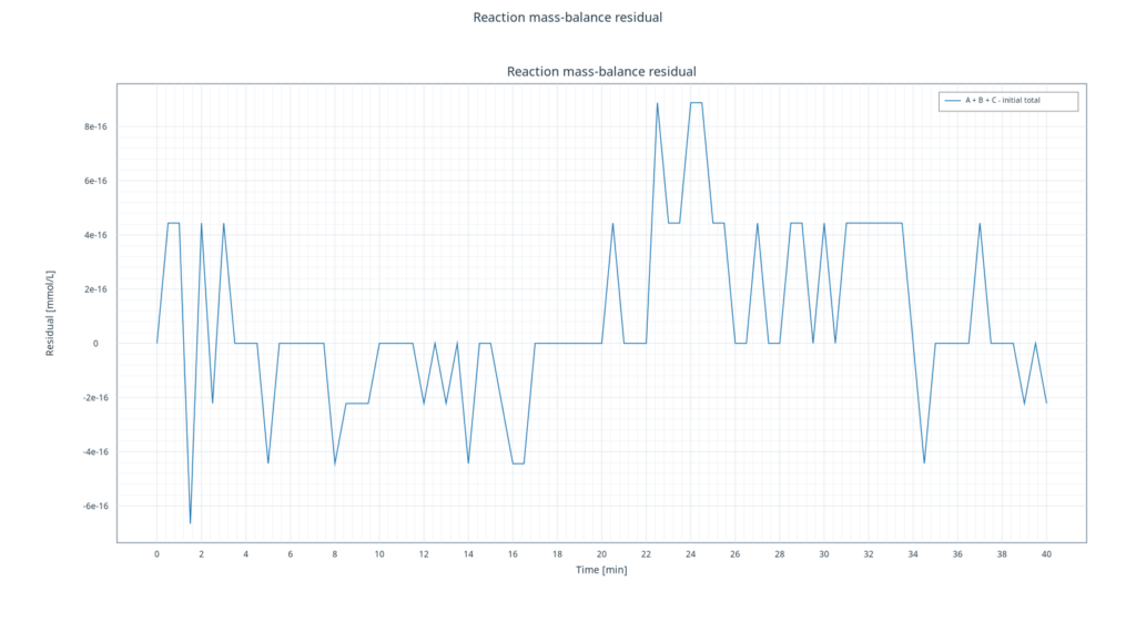
The third plot shows the residual \(A+B+C-A_0\), which stays close to zero in the corrected simulation.
What the public APIs do in this experiment
These APIs are not entirely new to the course. Here, however, they serve a specific scientific purpose: separating computation, data identity, and presentation. The ode45 solver and odeset belong to GNU Octave; they are not GX-TXT calls.
| API and operation | Purpose and check |
|---|---|
gxtxt_api_require({...}) | Checks before computation that the required API IDs are registered in the Script Bridge |
gxtxt_api_has_operation(id, op) | Checks that the requested operation is actually available |
CANONICAL_DATASET_API_v2 / list | Checks for existing reference Datasets or potential ID collisions |
CANONICAL_DATASET_API_v2 / read_range | Reads times and concentrations by Variable ID and row interval without opening private storage |
DATASET_PUBLICATION_API_v2 / publish_series_batch | Publishes multiple series with units and provenance in one atomic operation, then checks receipt.atomic and receipt.output_count |
PLOT_DATASET_API_v4 / new_spec, validate_spec, upsert_plot, render, artifacts | Defines, validates, registers, and renders persistent plots linked to Dataset IDs and Variable IDs |
A gxtxt_api_call invocation takes three arguments: the API identifier, the operation name, and a cell array of positional arguments. For example, {'lesson14_reference_b', {'time_min','concentration_mmol_L'}, 0, 81} requests 81 rows from the Dataset for species B, selecting two variables. Checking dimensions, increasing time coordinates, and units prevents meaningless numerical comparisons.
Solving ODEs through the public GX-TXT API: the intended route
So far, we have integrated the system with ode45, a native GNU Octave function. GX-TXT also provides the public NUMERIC_API_v1 interface, exposing the ode family and solve operation through the Script Bridge. Both approaches are worth understanding: the first teaches the language directly, while the second uses the framework’s numerical service through an API contract shared across supported languages.
Compatibility note for the version used in this lesson. In tests performed on November 14, 2026, with GX-TXT DEV112 Release 2 P008, the ODE call using a registered callback did not complete the Job: the Bridge reported GXTXT:ScriptBridge:Transport and BrokenPipeError during callback release. For this reason, the three executable scripts distributed here use ode45 and odeset, which were actually verified. The following example instead illustrates the public API contract documented on GitHub, but is not presented as code successfully tested on P008. The problem may have been fixed in later versions; readers reproducing the experiment should check their installed release.
Functions and their roles
| Public function / operation | Why it is needed |
|---|---|
gxtxt_api_require({'NUMERIC_API_v1'}) | Requires the numerical service to be available through the Bridge before execution. |
gxtxt_api_has_operation('NUMERIC_API_v1','foundation') | Checks that the entry point for foundation numerical operations is available. |
gxtxt_callback_register(rhs) | Registers a GNU Octave function that computes state derivatives; returns an opaque handle valid for the current execution. |
gxtxt_api_call('NUMERIC_API_v1','foundation',args) | Invokes ode/solve with the callback, time grid, initial state, and numerical options. |
gxtxt_callback_release(handle) | Releases the registered callback after the operation, following the Bridge lifecycle contract. |
The derivative function rhs(t,y) returns a three-component vector, one component per concentration. The Bridge does not transmit the function’s source code to an external interpreter: it uses an opaque identifier and invokes the function in the Octave runtime that started the script. The numerical provider’s callback path uses SciPy for integration; this should not be confused with calling ode45 directly in Octave.
A teaching example of the public API contract
This fragment shows how the service should be called once the issue has been confirmed fixed in the installed GX-TXT version. Code comments are in English, as in every script in this course. It does not replace the complete, validated scripts provided at the end of the article.
% GX-TXT public ODE example: documented interface, not tested in P008.
numeric_api = 'NUMERIC_API_v1';
gxtxt_api_require({numeric_api});
assert(gxtxt_api_has_operation(numeric_api, 'foundation'));

k1 = 0.24;
k2 = 0.075;
time_min = (0:0.5:40)';
initial_state = [2; 0; 0];
rhs = @(t,y) [-k1*y(1); k1*y(1)-k2*y(2); k2*y(2)];
callback = gxtxt_callback_register(rhs);

try
  solution = gxtxt_api_call(numeric_api, 'foundation', ...
    {'ode', 'solve', callback, time_min, initial_state, ...
     struct('reltol', 1e-8, 'abstol', 1e-10, 'max_step', 0.25)});
catch original_error
  % Preserve the initial failure if callback cleanup also fails.
  try
    gxtxt_callback_release(callback);
  catch cleanup_error
    fprintf(2, 'Callback cleanup failed: %s\n', cleanup_error.message);
  end_try_catch
  rethrow(original_error);
end_try_catch
gxtxt_callback_release(callback);

% Inspect the documented result structure before using its numeric fields.
disp(solution);
The positional arguments in the cell array are, in order: 'ode' (numerical family), 'solve' (action), the callback handle, requested times, the initial-state vector, and the options struct. reltol sets relative tolerance, abstol sets absolute tolerance, and max_step limits the maximum internal time step. These are not estimates of experimental uncertainty. The contract provides information about times, the calculated state, the number of returned values, and success/cancellation status; the actual result shape and fields must be checked against the installed release before publishing data.
The try/catch block also serves an educational purpose: an error during gxtxt_callback_release must not overwrite diagnostics from an earlier numerical failure. No nested Bridge calls should be made inside rhs: the Bridge waits for the callback to return the derivative vector before it can continue the active operation.
How to verify the fix in later releases
Once the installed version supports this route correctly, start with the documented scalar example y'=-2y, then repeat the three-species model. Before replacing ode45 in the main script, compare the curves with the analytical solution, verify that A+B+C=2 mmol/L holds within the chosen numerical tolerance, and check that callback release completes without errors in both normal and debugger execution modes.
Public documentation, pinned to the lesson’s source commit: Script Callback API v1, Octave Script Bridge API v1, and Numeric API v1.
Which persistent results are created
Script 00 publishes three analytical Datasets: lesson14_reference_a, lesson14_reference_b, and lesson14_reference_c. The corrected script publishes five derived Datasets: lesson14_ode_a, lesson14_ode_b, lesson14_ode_c, lesson14_mass_balance, and lesson14_b_absolute_error. Alongside the three concentrations, we therefore retain the mass-balance residual and the absolute error for intermediate B.
Batch publication does not replace verification: each series is read back through read_range and compared with its original values. Three persistent Plot Datasets show the complete kinetics, the analytical-versus-numerical comparison for B, and the conservation residual. Time variables use min as their unit; concentration and error variables use mmol/L. There is no need to generate standalone images with plotting commands outside GX-TXT.
Three scripts, three purposes
| Script | Contents | Result |
|---|---|---|
L14_00_Prepare_Analytical_Reference.m |
Analytical formula and atomic publication | 3 reference Datasets |
L14_01_Debug_Wrong_ODE_Sign.m |
Sign error, debugger, and mass balance | Intentionally failed Job; no Dataset |
L14_02_Kinetics_ODE_Correct.m |
ode45 integration, validation, publication, and plots |
5 derived Datasets and 3 Plot Datasets |
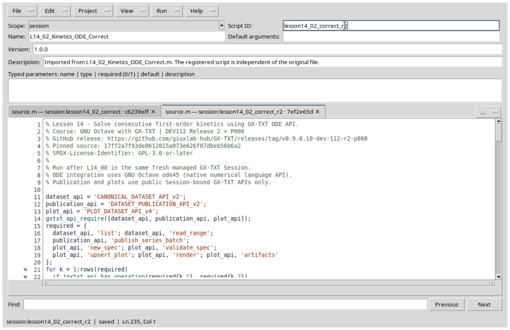
The three scripts must be imported into GX-TXT’s Octave Script Workspace and saved under distinct identifiers. First execute script 00, then run script 01 in Debug mode, and finally execute script 02. The second script fails by design: this is the condition that lets us diagnose an incorrect physical law. To repeat the entire experiment without Dataset ID collisions, create a new Session.

How to reproduce the lesson in GX-TXT
- Create a new Session using the GX-TXT version referenced below and open the Octave Script Workspace.
- Import and save the three
.mfiles using different names/IDs, retaining the original code. - Run
L14_00_Prepare_Analytical_Reference.mand confirm that three Datasets were published. - Run
L14_01_Debug_Wrong_ODE_Sign.min Debug mode and observe the deliberately triggered scientific failure. - Run
L14_02_Kinetics_ODE_Correct.m. Verify that five Datasets and three plots appear in the GX-TXT interface. - Open the Plot Datasets to compare the concentrations, check the overlap of the B curves, and observe a total residual close to zero.
To repeat the whole experiment without reusing the same IDs, start a new Session. The scripts do not write directly to the GX-TXT internal filesystem and do not require any CORE modifications.
Interpretation and limitations of the model
These data are synthetic, generated from a specified kinetic law. The rate constants are assumed known rather than estimated from measurements. We are not estimating uncertainties, confidence intervals, or parameters from an experiment: doing so would require a noise model and dedicated fitting procedures. Mass-balance validation checks the internal consistency of this model; it does not by itself prove that the mechanism describes a real chemical reaction.
One useful check is to rerun the calculation with a larger RelTol (thus reducing the requested accuracy) and compare the deviations; another is to change \(k_2\) and observe how the intermediate peak shifts.
Exercises
- Change the rate \(k_2\) and compare the time of the B maximum with the analytical expression.
- Set \([B](0)>0\): in this case you must recalculate the analytical solution, which will no longer coincide with the one given for the original initial conditions.
- Solve the problem with looser tolerances and compare the maximum error on the same time grid.
- Simulate a system in which species C is lost and explain why \(A+B+C\) is no longer conserved in the modified model.
- Explain why the units of \(k_1\) and \(k_2\) are inverse-time units and why concentration derivatives have units of \(\mathrm{mmol\,L^{-1}\,min^{-1}}\).
GX-TXT version and source references
The lesson was run with GX-TXT 0.9.8.10-dev-112 Release 2 P008 (a version pinned for reproducibility, verified on November 14, 2026), commit 17ff2a7f93de0612015a873e626f87dbeb56b6a2. The GX-TXT operations used are public and documented in the GitHub API contracts:
ode45 and odeset are native GNU Octave functions, not GX-TXT operations. In P008, the NUMERIC_API_v1 / foundation / ode/solve path with a registered callback did not pass testing, so the distributed scripts use the Octave method that was actually validated. Every Dataset and plot operation, however, uses GX-TXT’s public APIs exclusively. The section on the public ODE solver presents documentation and illustrative code that were not yet experimentally verified, separately from the results of the simulation that was actually run.
Materials
The three GNU Octave source files are available at the end of this article in expandable sections. All source-code comments are in English, and the educational explanations are now provided in English as well. The numerical results and plots can be regenerated within a new GX-TXT Session using the same parameters.
Complete GNU Octave scripts
Open the sections to inspect or copy the complete source files. All code comments are in English.
00 — L14_00_Prepare_Analytical_Reference.m
% Lesson 14 - Publish analytical reference kinetics for A -> B -> C.
% Course: GNU Octave with GX-TXT | DEV112 Release 2 + P008
% Source commit: 17ff2a7f93de0612015a873e626f87dbeb56b6a2
% SPDX-License-Identifier: GPL-3.0-or-later
%
% Run once in a fresh managed GX-TXT Session.
% These are deterministic reference profiles, not measured concentrations.

dataset_api = 'CANONICAL_DATASET_API_v2';
publication_api = 'DATASET_PUBLICATION_API_v2';
gxtxt_api_require({dataset_api, publication_api});
assert(gxtxt_api_has_operation(dataset_api, 'list'));
assert(gxtxt_api_has_operation(dataset_api, 'read_range'));
assert(gxtxt_api_has_operation(publication_api, 'publish_series_batch'));

k1_per_min = 0.24;
k2_per_min = 0.075;
initial_concentration = 2.0;
time_min = (0:0.5:40)';
n = numel(time_min);

% Closed-form solution of two consecutive first-order reactions.
reference_a = initial_concentration * exp(-k1_per_min * time_min);
reference_b = initial_concentration * k1_per_min / ...
  (k2_per_min - k1_per_min) .* ...
  (exp(-k1_per_min * time_min) - exp(-k2_per_min * time_min));
reference_c = initial_concentration - reference_a - reference_b;
assert(all(reference_a >= 0) && all(reference_b >= 0));
assert(all(reference_c > -1e-12));
assert(max(abs(reference_a + reference_b + reference_c - ...
               initial_concentration)) < 1e-12);

dataset_ids = {'lesson14_reference_a', ...
               'lesson14_reference_b', 'lesson14_reference_c'};
existing_ids = gxtxt_api_call(dataset_api, 'list', {});
for i = 1:numel(dataset_ids)
  if any(strcmp(existing_ids, dataset_ids{i}))
    error('Reference Dataset already exists: %s. Start a new Session.', ...
          dataset_ids{i});
  endif
endfor

time_variable = struct('variable_id', 'time_min', ...
  'name', 'time_min', 'display_label', 'Reaction time', ...
  'unit', 'min', 'dtype', 'float64', 'value_kind', 'number', ...
  'semantic_source', 'generator');
concentration_variable = struct('variable_id', 'concentration_mmol_L', ...
  'name', 'concentration_mmol_L', 'display_label', 'Concentration', ...
  'unit', 'mmol/L', 'dtype', 'float64', 'value_kind', 'number', ...
  'semantic_source', 'generator');
values = {reference_a, reference_b, reference_c};
species = {'A', 'B', 'C'};
series = cell(1, 3);
for i = 1:3
  meta = struct();
  meta.('kinetics.synthetic') = true;
  meta.('kinetics.reaction') = 'A -> B -> C';
  meta.('kinetics.k1_per_min') = k1_per_min;
  meta.('kinetics.k2_per_min') = k2_per_min;
  meta.('kinetics.initial_mmol_L') = initial_concentration;
  meta.('kinetics.species') = species{i};
  meta.('kinetics.method') = 'analytical_reference';
  series{i} = struct('dataset_id', dataset_ids{i}, ...
    'contract', 'table.generic', 'storage', 'auto', ...
    'x_values', time_min, 'y_values', values{i}, ...
    'x_variable', time_variable, 'y_variable', concentration_variable, ...
    'source', 'GX-TXT GNU Octave Lesson 14', ...
    'producer_version', '1.0.0', ...
    'provenance', 'Deterministic analytical consecutive reaction model', ...
    'notes', ['Analytical reference concentration for species ', species{i}], ...
    'structured_metadata', meta);
endfor

receipt = gxtxt_api_call(publication_api, 'publish_series_batch', ...
  {struct('series', {series})});
if !receipt.atomic || receipt.output_count != 3
  error('Atomic publication did not confirm three reference Datasets.');
endif
for i = 1:3
  saved = gxtxt_api_call(dataset_api, 'read_range', ...
    {dataset_ids{i}, {'time_min','concentration_mmol_L'}, 0, n});
  assert(max(abs(saved.time_min.values(:) - time_min)) < 1e-12);
  assert(max(abs(saved.concentration_mmol_L.values(:) - values{i})) < 1e-10);
endfor

peak_time_min = log(k1_per_min / k2_per_min) / ...
                (k1_per_min - k2_per_min);
peak_b_mmol_L = initial_concentration * k1_per_min / ...
  (k2_per_min - k1_per_min) * ...
  (exp(-k1_per_min * peak_time_min) - ...
   exp(-k2_per_min * peak_time_min));
fprintf('PASS: 3 analytical reference Datasets published.\n');
fprintf('k1 = %.3f min^-1, k2 = %.3f min^-1, initial = %.3f mmol/L.\n', ...
        k1_per_min, k2_per_min, initial_concentration);
fprintf('Analytical B peak: t = %.6f min, B = %.6f mmol/L.\n', ...
        peak_time_min, peak_b_mmol_L);
01 — L14_01_Debug_Wrong_ODE_Sign.m
% Lesson 14 - Debug a deliberately wrong sign in a kinetic ODE.
% Course: GNU Octave with GX-TXT | DEV112 Release 2 + P008
% Source commit: 17ff2a7f93de0612015a873e626f87dbeb56b6a2
% SPDX-License-Identifier: GPL-3.0-or-later
%
% Run after L14_00. Set a native debugger breakpoint near BREAKPOINT.
% An unphysical creation of matter MUST be detected as an expected failure.
% This script publishes no Dataset and no Plot Dataset.

dataset_api = 'CANONICAL_DATASET_API_v2';
gxtxt_api_require({dataset_api});
assert(gxtxt_api_has_operation(dataset_api, 'read_range'));

reference = gxtxt_api_call(dataset_api, 'read_range', ...
  {'lesson14_reference_a', {'time_min'}, 0, 81});
time_min = reference.time_min.values(:);
assert(numel(time_min) == 81 && all(diff(time_min) > 0));

k1 = 0.24;
k2 = 0.075;
initial_state = [2;0;0];

% INTENTIONAL ERROR: B incorrectly gains +k2*B instead of losing k2*B.
% The C product still gains k2*B, so the total concentration increases.
wrong_rhs = @(t,y) [-k1*y(1); k1*y(1) + k2*y(2); k2*y(2)];
% GNU Octave ode45 integrates the intentionally incorrect ODE.
% All GX-TXT access continues exclusively through its public APIs.
ode_options = odeset('RelTol', 1e-8, 'AbsTol', 1e-10, 'MaxStep', 0.25);
[solved_time, state_native] = ode45(wrong_rhs, time_min, initial_state, ...
                                   ode_options);
solution = struct('time', solved_time, 'state_real', state_native, ...
  'success', true, 'output_count', numel(solved_time));

state = solution.state_real;
if !solution.success || rows(state) != 81 || columns(state) != 3
  error('The GNU Octave ODE solver returned an unexpected result.');
endif
total = sum(state, 2);
maximum_conservation_error = max(abs(total - initial_state(1)));

% BREAKPOINT: inspect wrong_rhs, state, total,
% maximum_conservation_error, and initial_state.
fprintf('Final total = %.6f mmol/L; initial total = %.6f mmol/L.\n', ...
        total(end), initial_state(1));
fprintf('Maximum mass-balance error = %.6f mmol/L.\n', ...
        maximum_conservation_error);

% Expected FAILED Job: the flawed chemical model violates conservation.
if maximum_conservation_error > 1e-5
  error('GXTXT:Lesson14:MassConservation', ...
        'Conservation failed. Inspect the sign of the B consumption term.');
endif
error('Unexpected success: the intentional reaction-balance error escaped.');
02 — L14_02_Kinetics_ODE_Correct.m
% Lesson 14 - Solve kinetics with Octave ode45 and public GX-TXT Dataset/Plot APIs.
% Course: GNU Octave with GX-TXT | DEV112 Release 2 + P008
% GitHub release: https://github.com/giuxlab-hub/GX-TXT/releases/tag/v0.9.8.10-dev-112-r2-p008
% Pinned source: 17ff2a7f93de0612015a873e626f87dbeb56b6a2
% SPDX-License-Identifier: GPL-3.0-or-later
%
% Run after L14_00 in the same fresh managed GX-TXT Session.
% ODE integration uses GNU Octave ode45 (native numerical language API).
% Publication and plots use public Session-bound GX-TXT APIs only.

dataset_api = 'CANONICAL_DATASET_API_v2';
publication_api = 'DATASET_PUBLICATION_API_v2';
plot_api = 'PLOT_DATASET_API_v4';
gxtxt_api_require({dataset_api, publication_api, plot_api});
required = {
  dataset_api, 'list'; dataset_api, 'read_range';
  publication_api, 'publish_series_batch';
  plot_api, 'new_spec'; plot_api, 'validate_spec';
  plot_api, 'upsert_plot'; plot_api, 'render'; plot_api, 'artifacts'
};
for k = 1:rows(required)
  if !gxtxt_api_has_operation(required{k,1}, required{k,2})
    error('Missing public GX-TXT operation: %s/%s.', ...
          required{k,1}, required{k,2});
  endif
endfor

% Read each analytical reference through canonical Dataset and Variable IDs.
source_ids = {'lesson14_reference_a', ...
              'lesson14_reference_b', 'lesson14_reference_c'};
existing_ids = gxtxt_api_call(dataset_api, 'list', {});
n = 81;
time_min = [];
reference = zeros(n, 3);
for i = 1:3
  if !any(strcmp(existing_ids, source_ids{i}))
    error('Missing source Dataset %s. Execute L14_00 first.', source_ids{i});
  endif
  data = gxtxt_api_call(dataset_api, 'read_range', ...
    {source_ids{i}, {'time_min','concentration_mmol_L'}, 0, n});
  current_time = data.time_min.values(:);
  if numel(current_time) != n || any(diff(current_time) <= 0)
    error('Invalid strictly increasing time grid in source %s.', source_ids{i});
  endif
  if i == 1
    time_min = current_time;
  elseif max(abs(time_min - current_time)) > 1e-12
    error('Reference Datasets have incompatible time coordinates.');
  endif
  reference(:,i) = data.concentration_mmol_L.values(:);
endfor

% Define a coupled system dY/dt = F(t,Y) in physical concentration units.
% Reaction 1: A -> B, rate k1*A. Reaction 2: B -> C, rate k2*B.
k1 = 0.24;
k2 = 0.075;
initial_state = [2;0;0];
rhs = @(t,y) [-k1*y(1); k1*y(1) - k2*y(2); k2*y(2)];

% The ODE solver is GNU Octave's documented adaptive Runge-Kutta ode45.
% GX-TXT Dataset and Plot operations continue via public Script Bridge APIs.
ode_options = odeset('RelTol',1e-8,'AbsTol',1e-10,'MaxStep',0.25);
[solved_time_native, state_native] = ode45(rhs,time_min,initial_state, ...
                                          ode_options);
solution = struct('time',solved_time_native,'state_real',state_native, ...
  'success',true,'cancelled',false, ...
  'output_count',numel(solved_time_native),'method','ode45');

if !solution.success || solution.cancelled || ...
   solution.output_count != n
  error('The GNU Octave ODE solve did not complete on the requested time grid.');
endif
solved_time = solution.time(:);
state = solution.state_real;
if rows(state) != n || columns(state) != 3 || ...
   max(abs(solved_time - time_min)) > 1e-10 || ...
   any(!isfinite(state(:)))
  error('The ODE result does not match the source time and state dimensions.');
endif

% Independent scientific checks: reference solution and conserved total.
total = sum(state, 2);
conservation_error = total - initial_state(1);
model_difference = state - reference;
maximum_reference_error = max(abs(model_difference(:)));
maximum_conservation_error = max(abs(conservation_error));
minimum_state = min(state(:));
if minimum_state < -1e-9
  error('The calculated concentrations are negative beyond tolerance.');
endif
if maximum_reference_error > 1e-5
  error('Numerical solution differs from the analytical reference.');
endif
if maximum_conservation_error > 1e-6
  error('Reaction mass balance is not conserved.');
endif

% The intermediate B concentration has an exactly known peak time.
analytical_peak_time = log(k1/k2)/(k1-k2);
analytical_peak_b = initial_state(1)*k1/(k2-k1) * ...
  (exp(-k1*analytical_peak_time)-exp(-k2*analytical_peak_time));
[observed_peak_b,peak_index] = max(state(:,2));
sampled_peak_time = time_min(peak_index);
if abs(sampled_peak_time - analytical_peak_time) > 0.26
  error('The sampled intermediate peak does not match the kinetic model.');
endif

fprintf('ODE solver method: %s; output times: %d.\n', ...
        solution.method, solution.output_count);
fprintf('B peak: analytical t = %.6f min, sampled t = %.6f min.\n', ...
        analytical_peak_time, sampled_peak_time);
fprintf('Analytical B peak %.6f; sampled B peak %.6f mmol/L.\n', ...
        analytical_peak_b, observed_peak_b);
fprintf('Maximum reference error = %.3g mmol/L.\n', maximum_reference_error);
fprintf('Maximum mass-balance error = %.3g mmol/L.\n', ...
        maximum_conservation_error);

% Publish the three computed species plus two diagnostic series atomically.
derived_ids = {'lesson14_ode_a','lesson14_ode_b', 'lesson14_ode_c', ...
               'lesson14_mass_balance', 'lesson14_b_absolute_error'};
for i = 1:numel(derived_ids)
  if any(strcmp(existing_ids, derived_ids{i}))
    error('Derived Dataset already exists: %s. Use a fresh Session.', ...
          derived_ids{i});
  endif
endfor
time_variable = struct('variable_id', 'time_min', ...
  'name', 'time_min', 'display_label', 'Reaction time', ...
  'unit', 'min', 'dtype', 'float64', 'value_kind', 'number', ...
  'semantic_source', 'plugin');
concentration_variable = struct('variable_id', 'concentration_mmol_L', ...
  'name', 'concentration_mmol_L', 'display_label', 'Concentration', ...
  'unit', 'mmol/L', 'dtype', 'float64', 'value_kind', 'number', ...
  'semantic_source', 'plugin');
mass_variable = struct('variable_id', 'mass_balance_error_mmol_L', ...
  'name', 'mass_balance_error_mmol_L', ...
  'display_label', 'Mass balance error', ...
  'unit', 'mmol/L', 'dtype', 'float64', 'value_kind', 'number', ...
  'semantic_source', 'plugin');
difference_variable = struct('variable_id', 'abs_error_mmol_L', ...
  'name', 'abs_error_mmol_L', 'display_label', 'Absolute B error', ...
  'unit', 'mmol/L', 'dtype', 'float64', 'value_kind', 'number', ...
  'semantic_source', 'plugin');
values = {state(:,1),state(:,2),state(:,3), ...
          conservation_error,abs(model_difference(:,2))};
variable_defs = {concentration_variable,concentration_variable, ...
                 concentration_variable,mass_variable,difference_variable};
descriptions = {'ODE simulated A','ODE simulated B','ODE simulated C', ...
  'Conservation residual A + B + C - total initial', ...
  'Absolute ODE-minus-analytical error for B'};
series = cell(1,numel(derived_ids));
for i = 1:numel(derived_ids)
  meta = struct();
  meta.('kinetics.synthetic') = true;
  meta.('kinetics.model') = 'consecutive_first_order';
  meta.('kinetics.k1_per_min') = k1;
  meta.('kinetics.k2_per_min') = k2;
  meta.('kinetics.solver') = solution.method;
  meta.('kinetics.initial_mmol_L') = initial_state(1);
  meta.('kinetics.method') = descriptions{i};
  series{i} = struct('dataset_id',derived_ids{i}, ...
    'contract','table.generic','storage','auto', ...
    'x_values',time_min,'y_values',values{i}, ...
    'x_variable',time_variable,'y_variable',variable_defs{i}, ...
    'source','GX-TXT GNU Octave Lesson 14', ...
    'producer_version','1.0.0', ...
    'source_dataset_ids',{source_ids}, ...
    'provenance','GNU Octave ode45 with public GX-TXT Dataset services', ...
    'notes',descriptions{i},'structured_metadata',meta);
endfor
receipt = gxtxt_api_call(publication_api,'publish_series_batch', ...
  {struct('series',{series})});
if !receipt.atomic || receipt.output_count != numel(derived_ids)
  error('Atomic publication did not confirm five output Datasets.');
endif
for i = 1:numel(derived_ids)
  data = gxtxt_api_call(dataset_api, 'read_range', ...
    {derived_ids{i},{'time_min',variable_defs{i}.variable_id},0,n});
  actual = data.(variable_defs{i}.variable_id).values(:);
  if numel(actual) != n || max(abs(actual-values{i})) > 1e-9
    error('Published numerical data failed read-back verification.');
  endif
endfor

% Three persistent Plot Dataset v4 graphs refer to canonical variable IDs.
plot_definitions = {
  'lesson14_species_kinetics', 'Consecutive reaction: A, B, C', ...
    {'ODE A','ODE B','ODE C'}, derived_ids(1:3), ...
    {'concentration_mmol_L','concentration_mmol_L', ...
     'concentration_mmol_L'}, 'Concentration [mmol/L]';
  'lesson14_intermediate_comparison', 'Intermediate B: model validation', ...
    {'Numerical B','Analytical B'}, ...
    {'lesson14_ode_b','lesson14_reference_b'}, ...
    {'concentration_mmol_L','concentration_mmol_L'}, ...
    'Concentration [mmol/L]';
  'lesson14_conservation_error', 'Reaction mass-balance residual', ...
    {'A + B + C - initial total'}, {'lesson14_mass_balance'}, ...
    {'mass_balance_error_mmol_L'}, 'Residual [mmol/L]'
};
for p = 1:rows(plot_definitions)
  plot_id = plot_definitions{p,1};
  title_text = plot_definitions{p,2};
  labels = plot_definitions{p,3};
  dataset_list = plot_definitions{p,4};
  variable_list = plot_definitions{p,5};
  y_label = plot_definitions{p,6};
  spec = gxtxt_api_call(plot_api,'new_spec',{'plot.dataset.xy',title_text});
  panel = spec.panels{1};
  panel.id = ['panel_',num2str(p)];
  panel.title = title_text;
  panel.axes = struct('x', ...
    struct('label','Time [min]','scale','linear'), ...
    'y_left',struct('label',y_label,'scale','linear'));
  curves = cell(1,numel(labels));
  for k = 1:numel(labels)
    curves{k} = struct('id',['trace_',num2str(k)], ...
      'label',labels{k},'dataset_id',dataset_list{k}, ...
      'x_variable_id','time_min', ...
      'y_variable_id',variable_list{k},'axis','left','kind','line');
  endfor
  panel.series = curves;
  spec.panels = {panel};
  if !gxtxt_api_call(plot_api,'validate_spec',{spec})
    error('PlotSpec validation failed: %s.',plot_id);
  endif
  plot_ref = gxtxt_api_call(plot_api,'upsert_plot',{plot_id,spec});
  gxtxt_api_call(plot_api,'render',{plot_ref});
  plot_artifacts = gxtxt_api_call(plot_api,'artifacts',{plot_ref});
  fprintf('Created Plot Dataset: %s.\n', plot_id);
  disp(plot_artifacts);
endfor

fprintf('PASS: 5 canonical derived Datasets, 3 persistent plots.\n');
fprintf('PASS: GNU Octave ODE, analytical validation and conservation.\n');
Other steps of this project
- Lesson 01 — Your First GNU Octave Script in GX-TXT
- Lesson 02 — Variables, Data Types and Operators in GNU Octave with GX-TXT
- Lesson 03 — Vectors and Matrices in GNU Octave with GX-TXT: Temperature Measurement Analysis
- Lesson 04 — Conditions, Loops, and Functions. Simulating Newton’s Law of Cooling
- Lesson 05: Scientific Datasets and Variable IDs
- Lesson 06 — Selecting and Reading Experimental Data with GNU Octave and GX-TXT