

Lesson 16 — From UV-Vis Signals to a Kinetic Rate Constant: A Complete Scientific Project with GNU Octave and GX-TXT
Earlier lessons taught us how to represent data, solve linear systems, perform regressions, integrate differential equations and publish Datasets. We now bring these techniques together in a single experiment: we monitor a chemical transformation using dual-wavelength UV-Vis spectrophotometry, reconstruct the concentrations of the chemical species and test the kinetic law. The entire workflow takes place in a GX-TXT Session, using GNU Octave and the framework’s public APIs.
Reference version: GX-TXT 0.9.8.10-dev-112 Release 2 P009 — official GitHub release, sources at commit 059ff073eb43770292b6609f7c0cc3cbc811710d. The scripts are distributed under GPL-3.0-or-later; all source-code comments are in English.
Nature of the data. The absorbance values in this lesson are synthetic and deterministic: they simulate an experiment consistent with the Beer–Lambert law, with small mathematically defined perturbations. They are not laboratory measurements or experimental validation of a chemical reaction mechanism.
Learning objectives
By the end of this lesson, we will be able to link measurements, a physical model and persistent scientific results. We will revisit the organization of a program into stages, the matrix representation of a measurement model, solving several systems in one API call, regression with residual checks, integration with ode45, native debugging, and the preservation of results as Datasets and Plot Datasets.
Connecting the course: what is new in Lesson 16
Lessons 10–15 have already introduced the individual techniques. Here our main goal is to make them work together without losing the physical meaning of the data.
| Previously acquired knowledge | New application in the final project |
|---|---|
| Lesson 10 — regression and residuals | Estimate a kinetic parameter from concentrations that must first be recovered from optical signals |
| Lesson 11 — numerical calculus on time series | Keep observations aligned and units consistent across multiple processing stages |
| Lesson 12 — matrix rank, conditioning and linear systems | Solve 31 systems with the same matrix, using 31 columns of right-hand sides in one operation |
| Lesson 13 — signal sampling and representation | Treat two instrumental channels as synchronized observations of the same phenomenon |
Lesson 14 — anonymous functions, ode45 and conservation | Drive a dynamic model with estimated parameters, rather than setting every parameter before simulation |
| Lesson 15 — physical checks, units and independent validation | Organize checks before, during and after processing, through to scientific publication |
This is also a software-design exercise: we move from programs that perform a single calculation to a workflow with preconditions, postconditions and persistent scientific resources.
1. The scientific problem: monitoring an A → B reaction
Consider an irreversible first-order reaction:
Starting from \([A]_0=2.0\ \mathrm{mmol/L}\) and \([B]_0=0\), with a reference rate constant \(k=0.045\ \mathrm{min}^{-1}\), the exact solution is
The sum \([A](t)+[B](t)\) remains constant because matter is conserved. We use 31 observation times, from 0 to 60 minutes in two-minute intervals. During regression, we do not use the rate constant that generated the data: we estimate it from the absorbances, then compare the estimate against the known reference.
Why use two wavelengths?
A single absorbance measurement contains the contributions of all absorbing species. If both compounds absorb light, one observation is not sufficient to determine two separate concentrations. Measurements at 430 nm and 520 nm provide two independent equations.
For an optical path length of \(\ell=1\ \mathrm{cm}\), we define the molar absorptivity matrix
The Beer–Lambert law becomes
The rows represent wavelengths and the columns represent chemical species; keeping this order is essential. Absorbance is dimensionless (declared unit 1). The experiment works because the matrix has rank 2, so the two species can be distinguished.
The new scientific concept: a time-dependent inverse problem
The instrument measures two absorbances; the concentrations of A and B are not observed directly. Reconstructing them means solving an inverse problem: starting with measurable effects and inferring the quantities that produced them. The same Beer–Lambert relationship, used in the forward direction, lets us reconstruct the absorbances and check the answer.
Let \(Y\) denote the signals, \(C\) the concentrations and \(\Delta Y\) the small perturbations. The data-generation model is
To recover \(C\), the program uses \(\ell E\) and the observed \(Y\); it does not read the reference concentrations as inputs to the inverse solution. The reference Datasets are kept solely for comparison with the reconstructed solution. In this experiment, we assume that both species’ absorptivities and the optical path length are known; we neither estimate those coefficients nor propagate their uncertainties.
A further difficulty arises because these observations form a multichannel time series: all columns must correspond to the same instants. Two vectors with 31 values are not necessarily synchronized. This is why the final script checks the equality of the time coordinates, not just the sample count.
2. Preparing the first script: vectors, matrices and Datasets
The program L16_00_Prepare_UVVis_Kinetics.m constructs its time vector with (0:2:60)'; the apostrophe creates a column vector. The reference concentrations use exp and element-wise multiplication .*. The dot in front of the operator tells Octave to process every sample individually, rather than perform matrix multiplication.
The program then calculates the two absorbances and adds small, reproducible sinusoidal terms. These perturbations simulate signal imperfections but do not constitute a statistical model with a measured instrumental uncertainty.
Each series receives an explicit horizontal-variable definition, time_min, a variable_id for the measured quantity, units, synthetic provenance and scientific metadata. The script publishes five Datasets in a single operation:
| Dataset | Meaning |
|---|---|
lesson16_uvvis_430nm | Synthetic absorbance at 430 nm |
lesson16_uvvis_520nm | Synthetic absorbance at 520 nm |
lesson16_reference_A | Analytical concentration of A |
lesson16_reference_B | Analytical concentration of B |
lesson16_reference_total | Theoretical conserved total |
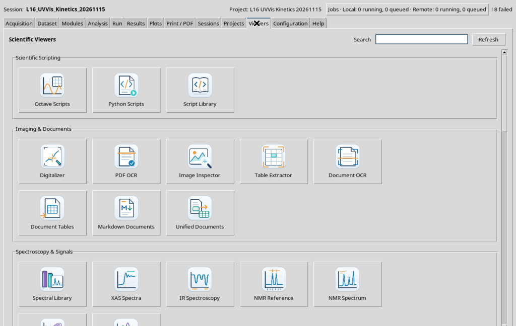
Once publication is complete, the script uses read_range to retrieve the five Datasets and compare them with the original arrays. The outcome is more than a numerical message: the resources remain associated with the Session and can be examined in GX-TXT Viewers.
3. Reasoning about matrix dimensions
In the final program, the absorbances are organized into a matrix \(\mathbf{Y}\) with dimensions \(2\times31\). Each row corresponds to a wavelength and each column to one observation time.
We must determine \(C\), whose first row contains A concentrations and whose second row contains B concentrations. GNU Octave distinguishes a nonconjugating transpose .' from a conjugate transpose ': they agree on real data but differ for complex matrices. Here [abs430.'; abs520.'] converts two columns of 31 observations into the required \(2\times31\) matrix.
We do not calculate the inverse of \(E\) explicitly. Through NUMERIC_API_v1/linear_matrix, we ask the CORE to examine rank and conditioning, then solve the system with multiple right-hand sides. A single call handles all 31 observations.
E = [0.75, 0.20; 0.12, 0.62];
Y = [abs430.'; abs520.'];
envelope_E = struct('real', E, 'imaginary', zeros(size(E)));
envelope_Y = struct('real', Y, 'imaginary', zeros(size(Y)));

check = gxtxt_api_call('NUMERIC_API_v1', 'linear_matrix', ...
  {'inspect', envelope_E, []});
solution = gxtxt_api_call('NUMERIC_API_v1', 'linear_matrix', ...
  {'solve', envelope_E, envelope_Y});
recovered_A = solution.value_real(1,:).';
recovered_B = solution.value_real(2,:).';
The real/imaginary envelope is the format specified by the public contract for transporting matrices through the Script Bridge. We do not need to know the CORE’s internal representation. The result is converted back into ordinary Octave arrays.
GNU Octave programming: cell arrays, structures and dynamic fields
Previous lessons introduced vectors, struct and cell array separately. The next step is to use them together to process several Datasets without duplicating the reading code. The third script uses the following pattern (an extract whose setup variables are already defined):
source_values = cell(1,numel(source_ids));
for j = 1:numel(source_ids)
  node = gxtxt_api_call(dataset_api,'read_range', ...
    {source_ids{j},{'time_min',source_y_ids{j}},0,n});
  source_values{j} = node.(source_y_ids{j}).values(:);
endfor
Understanding the syntax precisely is important:
| Octave expression | Meaning |
|---|---|
cell(1,numel(source_ids)) | Preallocates a cell array with one cell for each Dataset |
source_ids{j} | Extracts the contents of cell j, a string here; source_ids(j) would return a cell array |
node.(source_y_ids{j}) | Accesses a dynamic field of the structure, using the Variable ID read from the cell |
.values(:) | Extracts the values and converts them into a column vector, whatever their original orientation |
[abs430.'; abs520.'] | Converts two column vectors into two rows and concatenates them vertically |
result.value_real(1,:).' | Selects the first row of the solution and turns it back into a column vector |
The program also builds configuration tables as two-dimensional cell arrays: required{j,1} holds an API name, while required{j,2} identifies the operation to check; rows(required) gives the number of rows to process. The same pattern is used to define the five plots in plot_defs, separating the plot-specification data from the loop that creates the figures.
A more advanced detail concerns batch publication:
publish = gxtxt_api_call(publication_api,'publish_series_batch', ...
  {struct('series',{derived})});
Here derived is a cell array of seven specifications. The inner braces, {derived}, make the series field contain the entire collection, instead of constructing a separate structure for each cell. The outer braces wrap the positional argument passed to the public call. Understanding these nested levels matters when sending complex Octave structures through the Script Bridge.
4. Debugging: the scientific error of swapped wavelengths
The script L16_01_Debug_Swapped_Wavelengths.m deliberately contains an incorrect line:
wrong_absorbances = [A520.'; A430.'];The algorithm can run mathematically, but the signals are matched to the wrong rows of \(E\): a 520 nm response is interpreted as if it were measured at 430 nm, and vice versa. The program consequently produces impossible concentrations, including negative values. This is a concrete example of why a Job that runs without syntax errors does not automatically constitute a scientifically valid result.
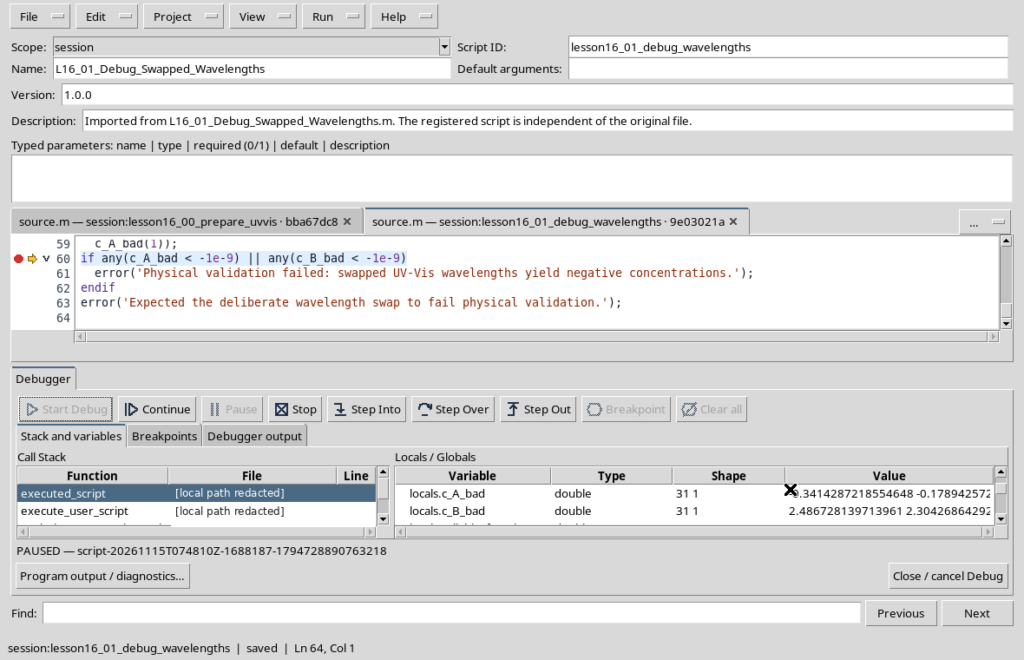
In the Octave Scripts Viewer, open Run → Debug Session script, select the script, set a breakpoint at line 60, and start the debugger. Examine c_A_bad and c_B_bad, as well as the wrong_absorbances matrix. The incorrectly reconstructed initial concentration of A is approximately −0.3414 mmol/L, while that of B exceeds 2.48 mmol/L: both violate the physical constraints of the chosen model.
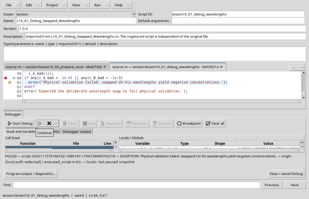
Press Continue. The concentration check deliberately causes the Job to fail. This is the correct behaviour: no derived Dataset is published from an inconsistent assignment of wavelengths.
5. Estimating the kinetic rate constant by regression
After correctly reconstructing the concentrations, we can test first-order kinetics. Taking the natural logarithm:
A plot of \(\ln[A]\) against \(t\) should be approximately linear. Its slope is \(-k\), while the intercept estimates \(\ln[A]_0\). We use GX-TXT’s public linear regression operation:
fit = gxtxt_api_call('NUMERIC_API_v1', 'linear_regression', ...
  {time_min, log(recovered_A), [], struct('intercept', true)});
k_estimated = -fit.slope;
A0_estimated = exp(fit.intercept);
R2 = fit.r_squared;
The empty vector [] occupies the weights-argument position: this is an ordinary, unweighted regression. struct('intercept',true) requests that the intercept be estimated too. Octave supplies log and exp; the public Numeric API estimates the coefficients.
The logarithmic transformation changes the interpretation of deviations: additive noise in absorbance space does not automatically become a homoscedastic error in \(\ln[A]\). We therefore treat this regression as an educational tool and state that limitation explicitly, without assigning confidence intervals that have not been calculated.
A new distinction: measurement error, estimation error and model error
In this processing chain, we make three different comparisons that should not be confused:
- The perturbations are added to the absorbances \(A_{430}\) and \(A_{520}\): they belong to signal space.
- The regression minimizes deviations of \(\ln[A]\) from a straight line: its \(R^2\) refers to log-concentration space.
- The final residuals compare reconstructed concentrations with ODE predictions: their RMS is expressed in mmol/L.
An \(R^2\) value close to 1 does not, by itself, guarantee that mass balance is respected or that the absorbance signals were assigned to the correct wavelengths. The three checks answer different questions.
The regression estimates both \(\hat{k}\) and \(\widehat{[A]_0}\); the initial condition \([B]_0=0\), however, is imposed by the chosen model, not determined by an additional fit. The reference value 0.045 appears in the synthetic-data generation and final benchmark, not as an input parameter to the regression. With actual measurements, the true value of \(k\) would normally be unknown, requiring an uncertainty and model-adequacy analysis.
6. Integrating differential equations with ode45
We return to Lesson 14. Using the parameters obtained from regression, we define an anonymous function in Octave:
rhs = @(t, y) [-k_estimated*y(1); k_estimated*y(1)];
options = odeset('RelTol',1e-10,'AbsTol',1e-11);
[t_model, state_model] = ode45(rhs, time_min, ...
  [A0_estimated; 0], options);
The vector y contains \([A]\) and \([B]\). The function rhs returns the two derivatives in the same order. ode45 is a native GNU Octave function, not a GX-TXT API: numerical integration is taught as part of the programming language. Through its public APIs, the framework handles Dataset inputs and result persistence.
The program compares the numerical solution for A with the exact formula \(A_0 e^{-kt}\) and checks that \(A+B\) remains constant. This double check helps identify errors in the differential model, initial conditions and array alignment.
7. Verifying the model, residuals and conservation of matter
A curve that appears to overlap the observations is not enough. The program separately verifies the quality of the reconstruction and the consistency of the equations:
- Positivity: A concentrations must be positive before taking their logarithm.
- Rank: the absorptivity matrix must allow the two species to be separated.
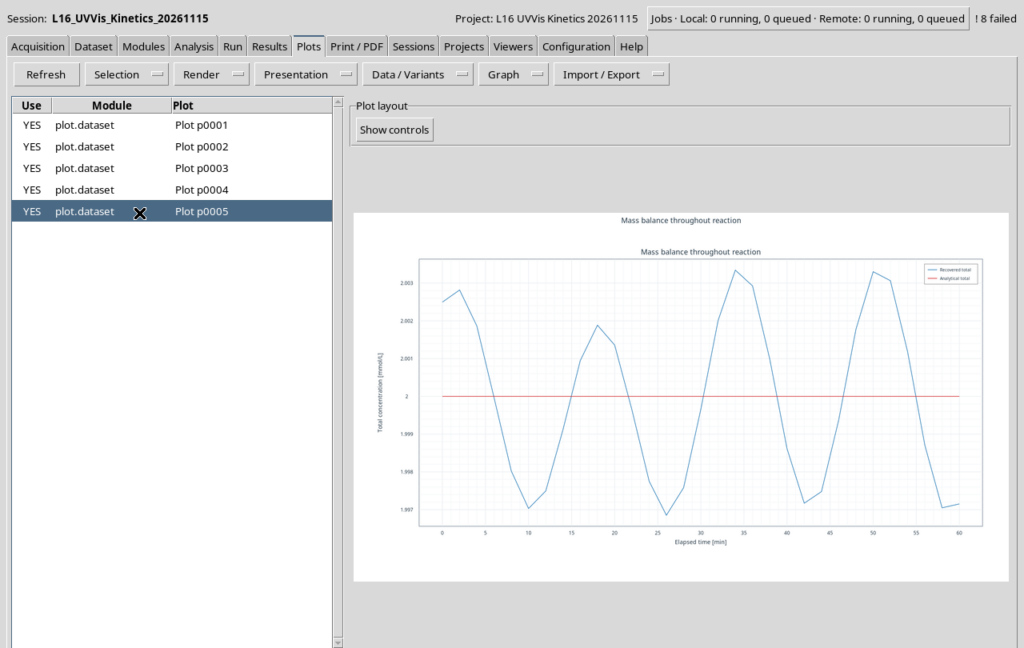
- Conservation: \([A]_{\mathrm{rec}}+[B]_{\mathrm{rec}}\) should stay close to \(2\ \mathrm{mmol/L}\).
- Residuals: for each species we calculate recovered-minus-predicted differences and their root-mean-square (RMS) value.
- Synthetic reference: the estimated \(k\) is compared with the value used to generate the data.
The following results were obtained for the case supplied with the scripts:
| Quantity | Result |
|---|---|
| Reference rate constant \(k\) | \(0.045000\ \mathrm{min}^{-1}\) |
| Estimated rate constant \(\hat{k}\) | \(0.04495570\ \mathrm{min}^{-1}\) |
| Estimated initial \([A]_0\) | \(1.99884590\ \mathrm{mmol/L}\) |
| Log-linear regression coefficient \(R^2\) | \(0.99996245\) |
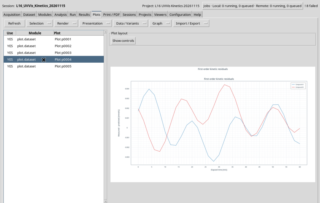
| Compound A residual RMS | \(0.00184381\ \mathrm{mmol/L}\) |
| Compound B residual RMS | \(0.00198044\ \mathrm{mmol/L}\) |
| Maximum total mass-balance deviation | \(0.00334298\ \mathrm{mmol/L}\) |
These values apply exclusively to the chosen synthetic model and must not be interpreted as guaranteed accuracy on experimental data.
Defensive programming: preconditions, invariants and postconditions
A reliable scientific script does more than check whether a Dataset exists. It must verify what the returned data mean and what shape they have. The third program applies checks at several levels:
| Level | Check performed | Consequence of a failure |
|---|---|---|
| Input | Datasets and Variable IDs present; strictly increasing time; matching time axes | Stop before combining incompatible series |
| Numeric structure | Rank-2 matrix, acceptable conditioning, output dimensions \(2\times31\) | Avoid misinterpreting components or columns |
| Physical meaning | Finite, physically admissible concentrations; \(\hat{k}>0\); conservation | Do not treat mathematically possible but implausible solutions as scientific results |
| Model | Agreement between ODE and analytical solution; residuals, \(R^2\), and synthetic-reference discrepancy | Distinguish calculation errors from reconstruction limitations |
| Persistence | Publication receipt and read-back through read_range | Verify that the stored result matches the calculated one |
Here is a dimension check from the corrected script:
if !isequal(size(result.value_real),[2,n]) || ...
   max(abs(result.value_imaginary(:))) > 1e-12
  error('Unexpected complex concentration result or response dimensions.');
endif
size returns array dimensions; isequal checks that they match exactly the expected shape. (:) allows all imaginary components to be examined as a single vector. The operator || is a short-circuit OR: if the first condition signals a problem, Octave need not evaluate the second. Constructs encountered earlier in the course—including numel, any, diff, isfinite, assert and error—now become part of one coherent validation strategy.
The program’s numeric thresholds are educational criteria, not universal metrology standards. For example, the condition-number limit (< 100), \(R^2>0.99\), the \(0.02\ \mathrm{mmol/L}\) limit for certain deviations, and the comparison of \(\hat{k}\) with the synthetic reference are intended to validate this particular example. They are not confidence intervals or uncertainty propagation. Moreover, checking conservation in the numerical ODE solution is distinct from checking the total concentration reconstructed from observations: the first tests the model, whereas the second tests the processed data.
8. GX-TXT public APIs: how and why we use them
This lesson clearly distinguishes between GNU Octave language operations and scientific services provided by the framework. All Dataset and plot operations use public APIs only, without opening CORE registry files or internal storage paths.
| Public API | Operation | Teaching purpose |
|---|---|---|
OCTAVE_SCRIPT_BRIDGE_API_v1 | gxtxt_api_require | Checks availability of required APIs before processing |
| Script Bridge | gxtxt_api_has_operation | Checks whether a provider exposes a specific operation |
| Script Bridge | gxtxt_api_call | Invokes a public operation with positional arguments wrapped in a cell array |
CANONICAL_DATASET_API_v2 | list | Discovers Datasets using stable logical IDs |
| Canonical Dataset v2 | read_range | Reads selected Variable IDs using an explicit zero-based start row and row count |
NUMERIC_API_v1 | linear_matrix('inspect') | Inspects the Beer–Lambert matrix rank and condition number |
| Numeric v1 | linear_matrix('solve') | Solves the system for 31 data columns in one call |
| Numeric v1 | linear_regression | Calculates the slope, intercept and regression \(R^2\) |
DATASET_PUBLICATION_API_v2 | publish_series_batch | Atomically publishes multiple series with units, metadata and provenance |
PLOT_DATASET_API_v4 | new_spec, validate_spec | Creates and validates a Dataset-driven plot specification |
| Plot Dataset v4 | upsert_plot, render, artifacts | Registers, renders and exposes the references for persistent plots |
For example, read_range receives {'lesson16_uvvis_430nm', {'time_min','absorbance_430_au'},0,31}. The first value is the Dataset ID; the inner cell array lists Variable IDs; 0 denotes the first row and 31 the number of observations. We do not supply CSV file paths, HDF5 references or internal handles. The Script Bridge converts the response into ordinary Octave structures.
With publish_series_batch we supply a collection of structures containing dataset_id, x_values, y_values, x_variable, y_variable, units, source information and structured_metadata. Atomic means that publishing the Datasets in a batch is treated as one coherent operation, rather than creating potentially incomplete results one at a time. The program checks the receipt and then reads the published Datasets back.
For plots, each trace is identified through dataset_id, x_variable_id and y_variable_id. Instead of saving PNGs generated by Octave as substitutes for scientific plots, we use the native Plot Dataset v4 family, which preserves references to the data.
Experiment architecture: from input Dataset to validated result
The novelty of GX-TXT integration lies in making the boundaries between program stages explicit:
- Logical acquisition.
listandread_rangeretrieve series by Dataset ID and Variable ID rather than filenames. The program checks the time alignment and finite values. - Inverse problem.
linear_matrix('inspect')checks the matrix;linear_matrix('solve')reconstructs 31 pairs of concentrations from the absorbances. - Identification and prediction.
linear_regressionestimates the parameters; Octave’sode45produces a model prediction distinct from pointwise absorbance inversion but based on parameters estimated from the same observations. - Validation and publication. Only after all checks does the script invoke
publish_series_batch. The receipt confirms the batch, andread_rangeverifies the seven derived Datasets. - Persistent visualization.
new_spec,validate_spec,upsert_plot,renderandartifactslink plots to the published Datasets instead of producing disconnected image files.
The code also distinguishes identifiers, values and provenance. For the seven derived Datasets, source_dataset_ids explicitly identifies the two absorbance Datasets used as reconstruction inputs. structured_metadata retains, among other quantities, \(\hat{k}\), \(\widehat{[A]_0}\), \(R^2\) and RMS values; these numbers need not be embedded in filenames or retrieved from internal CORE storage.
One final principle concerns controlled repeatability: the two scripts that publish Datasets first verify that their intended IDs do not already exist. Rerunning the experiment in the same Session risks an ID conflict; to repeat the entire workflow, create a new Session and retain the previous results. By contrast, upsert_plot registers or updates the plot specification associated with a Plot ID. These resource lifecycle semantics are different, and students should understand that distinction.
9. Five persistent scientific plots
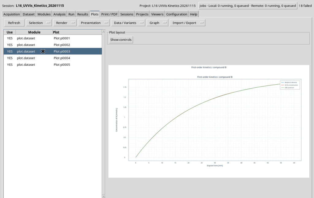
The third script, L16_02_UVVis_Kinetics_Correct.m, creates five separate plots, all accessible from the framework’s Plots tab. This separation is intentional: comparing absorbances, concentrations and residuals requires different scales and interpretations.
Absorbances at 430 and 520 nm
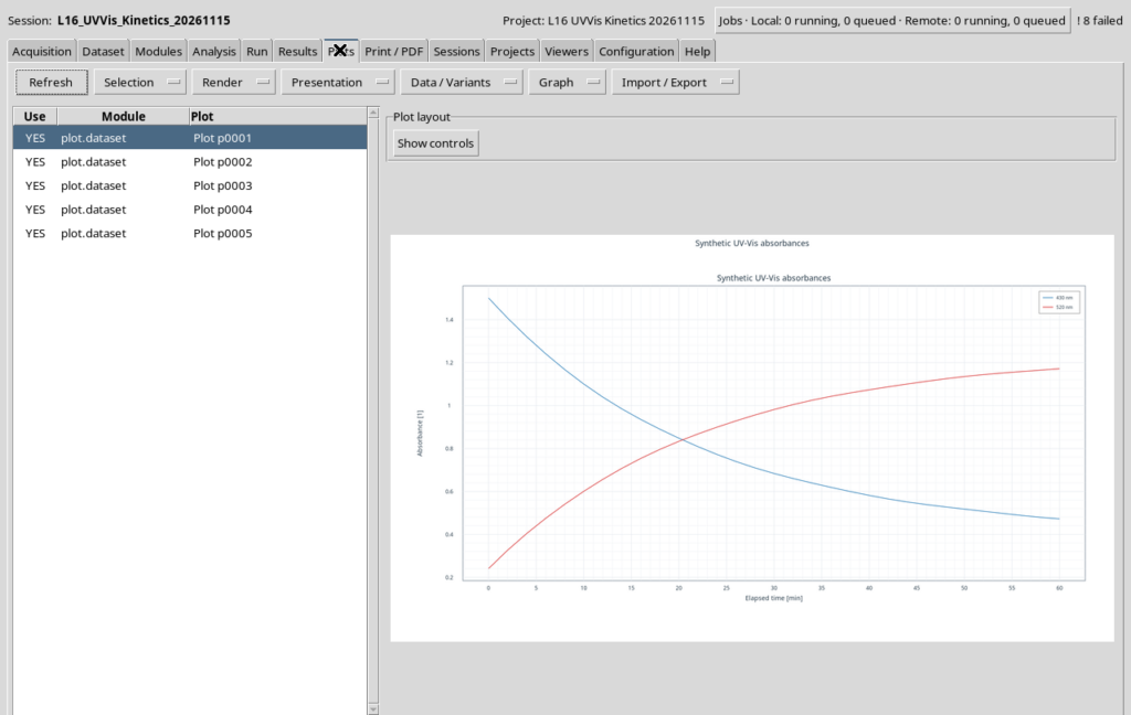
Reconstruction of compound A
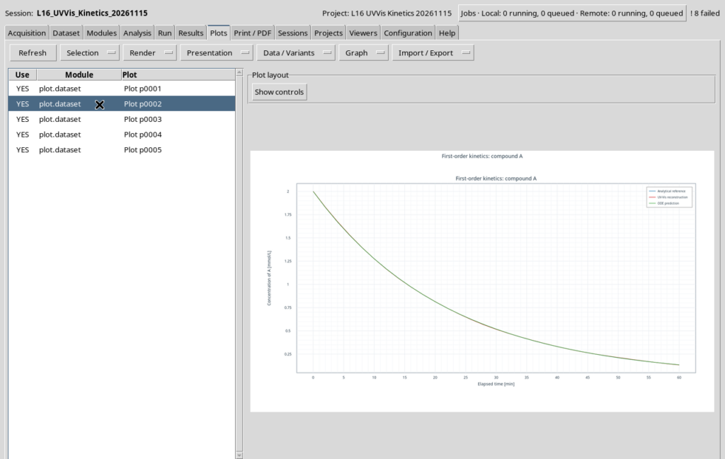
Reconstruction of compound B
Model residuals
Mass balance
10. Running the experiment in Octave Scripts Viewer
- Open a new Session inside a GX-TXT Project. The preparation scripts use create-only Dataset IDs, so a full repeat requires a fresh Session.
- In Viewers → Octave Scripts, import
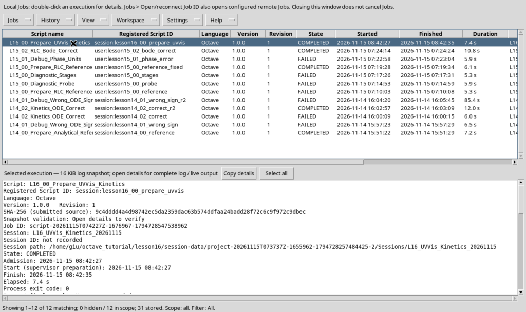
L16_00_Prepare_UVVis_Kinetics.m, assign a unique Script ID, save, and execute it using Run → Open Script Runner. Check theCOMPLETEDstatus and five source Datasets. - Import
L16_01_Debug_Swapped_Wavelengths.musing a second Script ID. Open Run → Debug Session script, set a breakpoint on line 60, inspect the variables, and press Continue. TheFAILEDJob is expected: it demonstrates physical validation. - Import
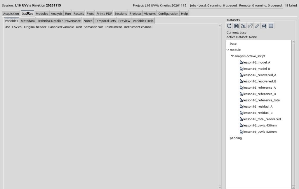
L16_02_UVVis_Kinetics_Correct.m, assign a third Script ID, save and execute it. Verify that the Job ends inCOMPLETED. - Open Dataset to examine the twelve Datasets and Plots to inspect the five native figures and their legends.
This procedure uses the Session, Dataset and Plot services already exposed through the GUI and the Script Bridge; no step requires modifying internal framework files.
11. Further exercises
- Change \(k\) to \(0.030\ \mathrm{min}^{-1}\) in the preparation script and compare the resulting curves and regression estimate in a separate Session.
- Make the two rows of the absorptivity matrix nearly proportional. Examine the condition number and explain why separating the species becomes less reliable.
- Increase the amplitude of the synthetic perturbations; examine the changes in \(R^2\), residual RMS and mass balance.
- Change the time grid: which
read_rangecalls and expected sample counts need updating? - Compare the log-linear approach against nonlinear fitting directly in absorbance space. Which assumptions about measurement noise change?
Final GNU Octave programming exercises
- Array orientation. In the debugger, compare
size(abs430),size(abs430.')andsize(measurements). Deliberately change a transpose, identify the diagnostic message, and restore the \(2\times31\) orientation. - Cell arrays and dynamic fields. Explain why
source_y_ids{j}differs fromsource_y_ids(j), and whynode.(source_y_ids{j}).values(:)makes the same loop work for five different variables. - Early checks. Make a copy of the script and add a time-axis check before solving the inverse problem. Explain the difference between rejecting inconsistent input and detecting excessive residuals after fitting.
- Modularization. As an extension, extract the time-axis consistency test into a reusable Octave function, specifying its inputs, outputs and error condition. Keep Dataset access exclusively within public APIs.
12. Conclusion: from calculation to a reproducible result
This experiment brings the learning sequence together: the matrix connects instrument signals to concentrations, regression supplies a kinetic parameter, differential-equation integration reconstructs its evolution over time, and consistency checks prevent the publication of physically impossible results.
The distinctive feature of integration with GX-TXT is that Datasets, units, provenance and plots remain scientific resources of the Session, rather than just numbers printed by a script. Octave language functions and the framework’s public APIs perform complementary, clearly identified roles.
Final assessment of the course
This lesson completes the 16-lesson introductory course. Starting with Octave syntax and vectors, we have reached an application that links simulated measurements, linear algebra, regression, dynamic models, physical validation, error handling and the publication of traceable results. The most important outcome is not a single kinetic rate constant, but the ability to explain and verify every step connecting an observation to that result.
The teaching project can be extended with further exercises and case studies; Lesson 16 completes the planned sequence without implying that GX-TXT development or scientific applications with GNU Octave stop here.
GX-TXT version and public documentation
Framework used: GX-TXT 0.9.8.10-dev-112 Release 2 P009, the version available on GitHub when the lesson was prepared. Verified source commit: 059ff073eb43770292b6609f7c0cc3cbc811710d. Reference date: November 15, 2026.
- Octave Script Bridge API v1
- Canonical Dataset API v2
- Dataset Publication API v2
- Plot Dataset API v4
- Numeric API v1
Teaching materials
The complete GNU Octave scripts, with English comments, are included in the downloadable Lesson 16 package: L16_00_Prepare_UVVis_Kinetics.m, L16_01_Debug_Swapped_Wavelengths.m and L16_02_UVVis_Kinetics_Correct.m. Their source code is also available in the expandable sections of this article.
Complete GNU Octave scripts
Expand each section to read and copy the complete source code.
Script 00 — L16_00_Prepare_UVVis_Kinetics.m
% Lesson 16 - Publish deterministic UV-Vis measurements and exact kinetic references.
% Course: GNU Octave with GX-TXT | DEV112 Release 2 + P009
% GitHub source commit: 059ff073eb43770292b6609f7c0cc3cbc811710d
% SPDX-License-Identifier: GPL-3.0-or-later
%
% Run this create-only preparation script in a fresh managed GX-TXT Session.
% All Datasets are created and verified through public GX-TXT APIs.
% The signals are synthetic, not experimental observations.

dataset_api = 'CANONICAL_DATASET_API_v2';
publication_api = 'DATASET_PUBLICATION_API_v2';
gxtxt_api_require({dataset_api, publication_api});
required = {dataset_api, 'list'; dataset_api, 'read_range'; ...
            publication_api, 'publish_series_batch'};
for j = 1:rows(required)
  if !gxtxt_api_has_operation(required{j,1}, required{j,2})
    error('Required public operation unavailable: %s/%s.', ...
          required{j,1}, required{j,2});
  endif
endfor

% A -> B first-order reaction. Concentrations are in mmol/L and time in min.
time_min = (0:2:60)';
initial_A_mmol_L = 2.0;
rate_min_inverse = 0.045;
path_length_cm = 1.0;
epsilon_L_mmol_cm = [0.75, 0.20; 0.12, 0.62];
n = numel(time_min);
assert(n == 31 && all(diff(time_min) > 0));
assert(rank(epsilon_L_mmol_cm) == 2);

% Exact analytical reference serves as ground truth for this synthetic example.
reference_A = initial_A_mmol_L .* exp(-rate_min_inverse .* time_min);
reference_B = initial_A_mmol_L - reference_A;
reference_total = reference_A + reference_B;

% Beer-Lambert absorbance at 430 and 520 nm, with fixed instrumental deviations.
% The deterministic perturbations make the example repeatable without a PRNG.
absorbance_430 = path_length_cm .* ...
  (epsilon_L_mmol_cm(1,1).*reference_A + epsilon_L_mmol_cm(1,2).*reference_B) ...
  + 0.0015 .* sin(0.40.*time_min) + 0.0008 .* cos(0.13.*time_min);
absorbance_520 = path_length_cm .* ...
  (epsilon_L_mmol_cm(2,1).*reference_A + epsilon_L_mmol_cm(2,2).*reference_B) ...
  + 0.0013 .* cos(0.37.*time_min + 0.2) - 0.0006 .* sin(0.16.*time_min);
assert(all(absorbance_430 > 0) && all(absorbance_520 > 0));
assert(max(abs(reference_total - initial_A_mmol_L)) < 1e-12);

dataset_ids = {'lesson16_uvvis_430nm','lesson16_uvvis_520nm', ...
               'lesson16_reference_A','lesson16_reference_B', ...
               'lesson16_reference_total'};
existing_ids = gxtxt_api_call(dataset_api, 'list', {});
for j = 1:numel(dataset_ids)
  if any(strcmp(existing_ids, dataset_ids{j}))
    error('Dataset already exists: %s. Use a fresh Session.', dataset_ids{j});
  endif
endfor

% Stable Variable IDs, explicit units and compatible dataset contracts.
time_variable = struct('variable_id','time_min','name','time_min', ...
  'display_label','Elapsed time','unit','min','dtype','float64', ...
  'value_kind','number','semantic_source','generator');
abs430_variable = struct('variable_id','absorbance_430_au', ...
  'name','absorbance_430_au','display_label','Absorbance at 430 nm', ...
  'unit','1','dtype','float64','value_kind','number', ...
  'semantic_source','generator');
abs520_variable = struct('variable_id','absorbance_520_au', ...
  'name','absorbance_520_au','display_label','Absorbance at 520 nm', ...
  'unit','1','dtype','float64','value_kind','number', ...
  'semantic_source','generator');
refA_variable = struct('variable_id','concentration_A_mmol_L', ...
  'name','concentration_A_mmol_L','display_label','Reference concentration A', ...
  'unit','mmol/L','dtype','float64','value_kind','number', ...
  'semantic_source','generator');
refB_variable = struct('variable_id','concentration_B_mmol_L', ...
  'name','concentration_B_mmol_L','display_label','Reference concentration B', ...
  'unit','mmol/L','dtype','float64','value_kind','number', ...
  'semantic_source','generator');
total_variable = struct('variable_id','total_mmol_L', ...
  'name','total_mmol_L','display_label','Reference total concentration', ...
  'unit','mmol/L','dtype','float64','value_kind','number', ...
  'semantic_source','generator');
values = {absorbance_430, absorbance_520, reference_A, reference_B, reference_total};
y_variables = {abs430_variable, abs520_variable, refA_variable, refB_variable, total_variable};
descriptions = {'Synthetic UV-Vis absorbance at 430 nm', ...
  'Synthetic UV-Vis absorbance at 520 nm', ...
  'Exact first-order analytical concentration of A', ...
  'Exact first-order analytical concentration of B', ...
  'Exact conserved molar concentration'};

series = cell(1,numel(dataset_ids));
for j = 1:numel(dataset_ids)
  metadata = struct();
  metadata.('lesson16.synthetic') = true;
  metadata.('lesson16.reaction') = 'A_to_B_first_order';
  metadata.('lesson16.rate_min_inverse') = rate_min_inverse;
  metadata.('lesson16.initial_A_mmol_L') = initial_A_mmol_L;
  metadata.('lesson16.path_length_cm') = path_length_cm;
  metadata.('lesson16.epsilon430_A') = epsilon_L_mmol_cm(1,1);
  metadata.('lesson16.epsilon430_B') = epsilon_L_mmol_cm(1,2);
  metadata.('lesson16.epsilon520_A') = epsilon_L_mmol_cm(2,1);
  metadata.('lesson16.epsilon520_B') = epsilon_L_mmol_cm(2,2);
  metadata.('lesson16.series_kind') = descriptions{j};
  series{j} = struct('dataset_id',dataset_ids{j}, ...
    'contract','table.generic','storage','auto', ...
    'x_values',time_min,'y_values',values{j}, ...
    'x_variable',time_variable,'y_variable',y_variables{j}, ...
    'source','GX-TXT GNU Octave Lesson 16','producer_version','1.0.0', ...
    'provenance','Deterministic first-order and Beer-Lambert synthetic generator', ...
    'notes',descriptions{j},'structured_metadata',metadata);
endfor
receipt = gxtxt_api_call(publication_api,'publish_series_batch', ...
  {struct('series',{series})});
if !receipt.atomic || receipt.output_count != numel(dataset_ids)
  error('Atomic publication did not confirm all five source Datasets.');
endif
for j = 1:numel(dataset_ids)
  check = gxtxt_api_call(dataset_api, 'read_range', ...
    {dataset_ids{j},{'time_min',y_variables{j}.variable_id},0,n});
  observed_time = check.time_min.values(:);
  observed_values = check.(y_variables{j}.variable_id).values(:);
  if numel(observed_values) != n || ...
     max(abs(observed_time-time_min)) > 1e-10 || ...
     max(abs(observed_values-values{j})) > 1e-10
    error('Public Dataset read-back failed for %s.',dataset_ids{j});
  endif
endfor
fprintf('PASS: 5 synthetic UV-Vis and analytical reference Datasets published.\n');
fprintf('Ground-truth first-order rate k=%.6f min^-1, initial A=%.3f mmol/L.\n', ...
  rate_min_inverse, initial_A_mmol_L);
fprintf('Measurement grid: %d points, from %.0f to %.0f min.\n', ...
  n,time_min(1),time_min(end));
Script 01 — L16_01_Debug_Swapped_Wavelengths.m
% Lesson 16 - Deliberately swap the wavelengths to debug a scientific error.
% Course: GNU Octave with GX-TXT | DEV112 Release 2 + P009
% GitHub source commit: 059ff073eb43770292b6609f7c0cc3cbc811710d
% SPDX-License-Identifier: GPL-3.0-or-later
%
% Run after L16_00 using Run > Debug Session script.
% Add a breakpoint before the physical consistency check and inspect c_A_bad.
% Expected outcome: FAILED, without publishing any new Dataset.

dataset_api = 'CANONICAL_DATASET_API_v2';
numeric_api = 'NUMERIC_API_v1';
gxtxt_api_require({dataset_api, ...
  'NUMERIC_API_v1@1:math.numeric+complex_linear_algebra'});
required = {dataset_api,'list'; dataset_api,'read_range'; ...
            numeric_api,'linear_matrix'};
for j = 1:rows(required)
  if !gxtxt_api_has_operation(required{j,1},required{j,2})
    error('Required public operation unavailable: %s/%s.', ...
      required{j,1},required{j,2});
  endif
endfor

source_ids = {'lesson16_uvvis_430nm','lesson16_uvvis_520nm'};
available_ids = gxtxt_api_call(dataset_api,'list',{});
for j = 1:numel(source_ids)
  if !any(strcmp(available_ids,source_ids{j}))
    error('Missing source Dataset %s. Run L16_00 first.',source_ids{j});
  endif
endfor
n = 31;
data430 = gxtxt_api_call(dataset_api,'read_range', ...
  {source_ids{1},{'time_min','absorbance_430_au'},0,n});
data520 = gxtxt_api_call(dataset_api,'read_range', ...
  {source_ids{2},{'time_min','absorbance_520_au'},0,n});
time_min = data430.time_min.values(:);
A430 = data430.absorbance_430_au.values(:);
A520 = data520.absorbance_520_au.values(:);
if numel(time_min) != n || ...
   max(abs(data520.time_min.values(:)-time_min)) > 1e-12
  error('Time axes are not aligned.');
endif

% Correct molar absorptivities, with rows in the order 430 nm and 520 nm.
epsilon = [0.75,0.20;0.12,0.62];
matrix_node = struct('real',epsilon,'imaginary',zeros(size(epsilon)));

% BUG: the measured 520 nm signal is placed in the 430 nm row, and vice versa.
wrong_absorbances = [A520.'; A430.'];
bad_rhs = struct('real',wrong_absorbances, ...
                 'imaginary',zeros(size(wrong_absorbances)));
result = gxtxt_api_call(numeric_api,'linear_matrix', ...
  {'solve',matrix_node,bad_rhs});
c_A_bad = result.value_real(1,:).';
c_B_bad = result.value_real(2,:).';

% BREAKPOINT: inspect wrong_absorbances, c_A_bad(1), min(c_A_bad), c_B_bad.
% A negative concentration is not an acceptable result of this model.
fprintf('Swapped wavelengths: initial reconstructed A=%.6f mmol/L.\n', ...
  c_A_bad(1));
if any(c_A_bad < -1e-9) || any(c_B_bad < -1e-9)
  error('Physical validation failed: swapped UV-Vis wavelengths yield negative concentrations.');
endif
error('Expected the deliberate wavelength swap to fail physical validation.');
Script 02 — L16_02_UVVis_Kinetics_Correct.m
% Lesson 16 - Complete synthetic UV-Vis kinetics analysis with GX-TXT.
% Course: GNU Octave with GX-TXT | DEV112 Release 2 + P009
% GitHub source commit: 059ff073eb43770292b6609f7c0cc3cbc811710d
% SPDX-License-Identifier: GPL-3.0-or-later
%
% Run after L16_00 in a managed GX-TXT Session.
% The Dataset, numerical linear/regression, publication and plot operations
% all use versioned public GX-TXT APIs through the Octave Script Bridge.
% ode45 and the array expressions are GNU Octave language operations.

dataset_api = 'CANONICAL_DATASET_API_v2';
numeric_api = 'NUMERIC_API_v1';
publication_api = 'DATASET_PUBLICATION_API_v2';
plot_api = 'PLOT_DATASET_API_v4';
gxtxt_api_require({dataset_api, ...
  'NUMERIC_API_v1@1:math.numeric+complex_linear_algebra', ...
  publication_api,plot_api});
required = {dataset_api,'list';dataset_api,'read_range'; ...
  numeric_api,'linear_matrix';numeric_api,'linear_regression'; ...
  publication_api,'publish_series_batch'; ...
  plot_api,'new_spec';plot_api,'validate_spec'; ...
  plot_api,'upsert_plot';plot_api,'render';plot_api,'artifacts'};
for j=1:rows(required)
  if !gxtxt_api_has_operation(required{j,1},required{j,2})
    error('Missing public GX-TXT operation: %s/%s.',required{j,1},required{j,2});
  endif
endfor

% 1. Read five canonical source Datasets by stable Dataset and Variable IDs.
source_ids={'lesson16_uvvis_430nm','lesson16_uvvis_520nm', ...
            'lesson16_reference_A','lesson16_reference_B', ...
            'lesson16_reference_total'};
source_y_ids={'absorbance_430_au','absorbance_520_au', ...
              'concentration_A_mmol_L','concentration_B_mmol_L','total_mmol_L'};
existing_ids=gxtxt_api_call(dataset_api,'list',{});
for j=1:numel(source_ids)
  if !any(strcmp(existing_ids,source_ids{j}))
    error('Missing source Dataset %s. Run L16_00 first.',source_ids{j});
  endif
endfor
n=31;
source_values=cell(1,numel(source_ids));
for j=1:numel(source_ids)
  node=gxtxt_api_call(dataset_api,'read_range', ...
    {source_ids{j},{'time_min',source_y_ids{j}},0,n});
  tx=node.time_min.values(:);
  if j==1
    time_min=tx;
  elseif numel(tx)!=n || max(abs(tx-time_min))>1e-12
    error('Source time axes differ; the kinetic model needs aligned observations.');
  endif
  source_values{j}=node.(source_y_ids{j}).values(:);
  if numel(source_values{j})!=n || any(!isfinite(source_values{j}))
    error('Nonfinite or incomplete source values in %s.',source_ids{j});
  endif
endfor
if numel(time_min)!=n || any(diff(time_min)<=0)
  error('The time grid is not strictly increasing.');
endif
abs430=source_values{1};
abs520=source_values{2};
reference_A=source_values{3};
reference_B=source_values{4};
reference_total=source_values{5};
assert(max(abs(reference_A+reference_B-reference_total))<1e-12);

% 2. Beer-Lambert matrix: rows are wavelengths, columns are compounds A and B.
% E has units L/(mmol*cm), path length has cm and concentrations are mmol/L.
path_length_cm=1.0;
epsilon_L_mmol_cm=[0.75,0.20;0.12,0.62];
design=epsilon_L_mmol_cm*path_length_cm;
measurements=[abs430.';abs520.'];
design_node=struct('real',design,'imaginary',zeros(size(design)));
rhs_node=struct('real',measurements,'imaginary',zeros(size(measurements)));
matrix_info=gxtxt_api_call(numeric_api,'linear_matrix', ...
  {'inspect',design_node,[]});
if matrix_info.rank!=2 || matrix_info.condition_number>=100
  error('The Beer-Lambert matrix is rank-deficient or poorly conditioned.');
endif

% 3. Solve the two-by-two system for all times in a single multi-RHS call.
result=gxtxt_api_call(numeric_api,'linear_matrix', ...
  {'solve',design_node,rhs_node});
if !isequal(size(result.value_real),[2,n]) || ...
   max(abs(result.value_imaginary(:)))>1e-12
  error('Unexpected complex concentration result or response dimensions.');
endif
recovered_A=result.value_real(1,:).';
recovered_B=result.value_real(2,:).';
if any(recovered_A<=0) || any(recovered_B<0)
  error('Negative or zero physical concentrations: check wavelength ordering.');
endif
reconstruction=design*[recovered_A.';recovered_B.'];
if max(abs(reconstruction(:)-measurements(:)))>1e-10
  error('Beer-Lambert algebraic reconstruction failed.');
endif
total_recovered=recovered_A+recovered_B;
max_mass_error=max(abs(total_recovered-reference_total));

% 4. Estimate first-order rate by public regression of ln([A]) vs time.
% The log-linear approximation is educational; noise is in absorbance space.
fit=gxtxt_api_call(numeric_api,'linear_regression', ...
  {time_min,log(recovered_A),[],struct('intercept',true)});
estimated_k_min_inverse=-fit.slope;
estimated_A0_mmol_L=exp(fit.intercept);
if estimated_k_min_inverse<=0 || estimated_A0_mmol_L<=0 || ...
   !isfinite(estimated_k_min_inverse) || fit.r_squared<0.99
  error('Regression did not yield a plausible first-order kinetic law.');
endif

% 5. Integrate the coupled kinetic system with GNU Octave ode45.
% dnA/dt = -k*A, dnB/dt = k*A; initial B is zero in the chosen model.
rhs=@(t,y) [-estimated_k_min_inverse*y(1);estimated_k_min_inverse*y(1)];
ode_options=odeset('RelTol',1e-10,'AbsTol',1e-11);
[time_solution,state_solution]=ode45(rhs,time_min, ...
  [estimated_A0_mmol_L;0],ode_options);
if numel(time_solution)!=n || max(abs(time_solution-time_min))>1e-8
  error('ode45 did not return the requested observation grid.');
endif
model_A=state_solution(:,1);
model_B=state_solution(:,2);
analytic_A=estimated_A0_mmol_L.*exp(-estimated_k_min_inverse.*time_min);
if max(abs(model_A-analytic_A))>1e-7 || ...
   max(abs(model_A+model_B-estimated_A0_mmol_L))>1e-8
  error('ODE solution violates the independent analytical or mass-balance test.');
endif

% 6. Quantify model residuals and compare with synthetic ground truth.
residual_A=recovered_A-model_A;
residual_B=recovered_B-model_B;
rms_A=sqrt(mean(residual_A.^2));
rms_B=sqrt(mean(residual_B.^2));
true_k_min_inverse=0.045;
max_reference_error=max([abs(recovered_A-reference_A); ...
                         abs(recovered_B-reference_B)]);
if max_mass_error>0.02 || max_reference_error>0.02 || ...
   rms_A>0.02 || rms_B>0.02 || ...
   abs(estimated_k_min_inverse-true_k_min_inverse)>0.005
  error('Kinetic reconstruction failed the specified scientific validation.');
endif
fprintf('Estimated k=%.8f min^-1; A(0)=%.6f mmol/L; R^2=%.8f.\n', ...
  estimated_k_min_inverse,estimated_A0_mmol_L,fit.r_squared);
fprintf('Residual RMS A=%.8f, B=%.8f mmol/L; max mass error=%.8f mmol/L.\n', ...
  rms_A,rms_B,max_mass_error);
fprintf('Design rank=%d; condition number=%.6f.\n', ...
  matrix_info.rank,matrix_info.condition_number);

% 7. Publish seven derived canonical series as one atomic GX-TXT operation.
derived_ids={'lesson16_recovered_A','lesson16_recovered_B', ...
  'lesson16_model_A','lesson16_model_B', ...
  'lesson16_residual_A','lesson16_residual_B', ...
  'lesson16_total_recovered'};
for j=1:numel(derived_ids)
  if any(strcmp(existing_ids,derived_ids{j}))
    error('Derived Dataset already exists: %s. Use a new Session.',derived_ids{j});
  endif
endfor
time_var=struct('variable_id','time_min','name','time_min', ...
  'display_label','Elapsed time','unit','min','dtype','float64', ...
  'value_kind','number','semantic_source','plugin');
A_var=struct('variable_id','concentration_A_mmol_L', ...
  'name','concentration_A_mmol_L','display_label','Concentration of A', ...
  'unit','mmol/L','dtype','float64','value_kind','number', ...
  'semantic_source','plugin');
B_var=struct('variable_id','concentration_B_mmol_L', ...
  'name','concentration_B_mmol_L','display_label','Concentration of B', ...
  'unit','mmol/L','dtype','float64','value_kind','number', ...
  'semantic_source','plugin');
resA_var=struct('variable_id','residual_A_mmol_L', ...
  'name','residual_A_mmol_L','display_label','Residual of A', ...
  'unit','mmol/L','dtype','float64','value_kind','number', ...
  'semantic_source','plugin');
resB_var=struct('variable_id','residual_B_mmol_L', ...
  'name','residual_B_mmol_L','display_label','Residual of B', ...
  'unit','mmol/L','dtype','float64','value_kind','number', ...
  'semantic_source','plugin');
total_var=struct('variable_id','total_mmol_L', ...
  'name','total_mmol_L','display_label','Total recovered concentration', ...
  'unit','mmol/L','dtype','float64','value_kind','number', ...
  'semantic_source','plugin');
derived_y={recovered_A,recovered_B,model_A,model_B,residual_A,residual_B, ...
  total_recovered};
derived_vars={A_var,B_var,A_var,B_var,resA_var,resB_var,total_var};
notes={'Reconstructed A from the two UV-Vis wavelengths', ...
       'Reconstructed B from the two UV-Vis wavelengths', ...
       'Coupled first-order ODE prediction for A', ...
       'Coupled first-order ODE prediction for B', ...
       'Reconstructed minus predicted A concentration', ...
       'Reconstructed minus predicted B concentration', ...
       'Recovered A+B mass-balance trace'};
derived=cell(1,numel(derived_ids));
for j=1:numel(derived_ids)
  meta=struct();
  meta.('lesson16.synthetic_inputs')=true;
  meta.('lesson16.analysis')='BeerLambert_linear_solve_log_regression_ode45';
  meta.('lesson16.k_fit_min_inverse')=estimated_k_min_inverse;
  meta.('lesson16.initial_fit_mmol_L')=estimated_A0_mmol_L;
  meta.('lesson16.fit_r_squared')=fit.r_squared;
  meta.('lesson16.max_mass_error_mmol_L')=max_mass_error;
  meta.('lesson16.rms_A_mmol_L')=rms_A;
  meta.('lesson16.rms_B_mmol_L')=rms_B;
  meta.('lesson16.output_role')=notes{j};
  derived{j}=struct('dataset_id',derived_ids{j}, ...
    'contract','table.generic','storage','auto', ...
    'x_values',time_min,'y_values',derived_y{j}, ...
    'x_variable',time_var,'y_variable',derived_vars{j}, ...
    'source','GX-TXT GNU Octave Lesson 16', ...
    'producer_version','1.0.0', ...
    'source_dataset_ids',{source_ids(1:2)}, ...
    'provenance','Public linear_matrix, linear_regression and GNU Octave ode45', ...
    'notes',notes{j},'structured_metadata',meta);
endfor
publish=gxtxt_api_call(publication_api,'publish_series_batch', ...
  {struct('series',{derived})});
if !publish.atomic || publish.output_count!=numel(derived_ids)
  error('Atomic publication did not confirm seven derived Datasets.');
endif
for j=1:numel(derived_ids)
  check=gxtxt_api_call(dataset_api,'read_range', ...
    {derived_ids{j},{'time_min',derived_vars{j}.variable_id},0,n});
  yy=check.(derived_vars{j}.variable_id).values(:);
  if numel(yy)!=n || max(abs(yy-derived_y{j}))>1e-9 || ...
     max(abs(check.time_min.values(:)-time_min))>1e-9
    error('Canonical read-back mismatch for Dataset %s.',derived_ids{j});
  endif
endfor

% 8. Create five persistent native GX-TXT Plot Dataset v4 figures.
% All visible traces resolve stable Dataset IDs and Variable IDs.
plot_defs={
 'lesson16_absorbances','Synthetic UV-Vis absorbances', ...
 {'430 nm','520 nm'}, ...
 {'lesson16_uvvis_430nm','lesson16_uvvis_520nm'}, ...
 {'absorbance_430_au','absorbance_520_au'},'Absorbance [1]';
 'lesson16_kinetics_A','First-order kinetics: compound A', ...
 {'Analytical reference','UV-Vis reconstruction','ODE prediction'}, ...
 {'lesson16_reference_A','lesson16_recovered_A','lesson16_model_A'}, ...
 {'concentration_A_mmol_L','concentration_A_mmol_L','concentration_A_mmol_L'}, ...
 'Concentration of A [mmol/L]';
 'lesson16_kinetics_B','First-order kinetics: compound B', ...
 {'Analytical reference','UV-Vis reconstruction','ODE prediction'}, ...
 {'lesson16_reference_B','lesson16_recovered_B','lesson16_model_B'}, ...
 {'concentration_B_mmol_L','concentration_B_mmol_L','concentration_B_mmol_L'}, ...
 'Concentration of B [mmol/L]';
 'lesson16_concentration_residuals','First-order kinetic residuals', ...
 {'Compound A','Compound B'}, ...
 {'lesson16_residual_A','lesson16_residual_B'}, ...
 {'residual_A_mmol_L','residual_B_mmol_L'},'Measured - predicted [mmol/L]';
 'lesson16_mass_balance','Mass balance throughout reaction', ...
 {'Recovered total','Analytical total'}, ...
 {'lesson16_total_recovered','lesson16_reference_total'}, ...
 {'total_mmol_L','total_mmol_L'},'Total concentration [mmol/L]'
};
for p=1:rows(plot_defs)
  plot_id=plot_defs{p,1};
  plot_title=plot_defs{p,2};
  labels=plot_defs{p,3};
  dataset_list=plot_defs{p,4};
  variable_list=plot_defs{p,5};
  plot_spec=gxtxt_api_call(plot_api,'new_spec',{'plot.dataset.xy',plot_title});
  panel=plot_spec.panels{1};
  panel.id=['kinetic_panel_',num2str(p)];
  panel.title=plot_title;
  panel.axes=struct('x',struct('label','Elapsed time [min]','scale','linear'), ...
    'y_left',struct('label',plot_defs{p,6},'scale','linear'));
  curves=cell(1,numel(labels));
  for j=1:numel(labels)
    curves{j}=struct('id',['trace_',num2str(j)],'label',labels{j}, ...
      'dataset_id',dataset_list{j},'x_variable_id','time_min', ...
      'y_variable_id',variable_list{j},'axis','left','kind','line');
  endfor
  panel.series=curves;
  plot_spec.panels={panel};
  if !gxtxt_api_call(plot_api,'validate_spec',{plot_spec})
    error('Plot Dataset specification invalid: %s.',plot_id);
  endif
  plot_ref=gxtxt_api_call(plot_api,'upsert_plot',{plot_id,plot_spec});
  gxtxt_api_call(plot_api,'render',{plot_ref});
  artifacts=gxtxt_api_call(plot_api,'artifacts',{plot_ref});
  fprintf('Created persistent GX-TXT plot: %s.\n',plot_id);
endfor
fprintf('PASS: 7 derived canonical Datasets, 5 native plots, 1 validated kinetic model.\n');
Other steps of this project
- Lesson 01 — Your First GNU Octave Script in GX-TXT
- Lesson 02 — Variables, Data Types and Operators in GNU Octave with GX-TXT
- Lesson 03 — Vectors and Matrices in GNU Octave with GX-TXT: Temperature Measurement Analysis
- Lesson 04 — Conditions, Loops, and Functions. Simulating Newton’s Law of Cooling
- Lesson 05: Scientific Datasets and Variable IDs
- Lesson 06 — Selecting and Reading Experimental Data with GNU Octave and GX-TXT