

NumPy Arrays, Dtype and Shape
Scientific Python in GX-TXT · Module 3 · Lesson 13
In the previous module we read a Dataset for blocks. Now we see how the numerical values come to Python and introduce NumPy arrays: containers designed for multidimensional numerical data and efficient operations.
Objectives: distinguish a list from a ndarray; read shape, ndim, size and dtype; recognize a column vector; understand the difference between logical order and layout in memory.
Prerequisites: lists, Dataset and reading with read_range of previous lessons; NumPy available in the interpreter configured in GX-TXT.
From a list to an array
A Python list can contain objects of different types. An array NumPy (ndarray) describes a grid of elements, generally all with the same numeric type, and keeps information about form and layout of data:
import numpy as np

values = np.array([1.2, 1.5, 1.3, 1.6])
print(values)
np is a conventional name chosen in import. The code builds an array of four synthetic values; they are not real measures. Array operations can be applied to entire sets of elements, but vectorization and broadcasting will be faced later.
np.asarray(oggetto) gets a representation as an array when possible. It can reuse a compatible array instead of copying it: do not assume it always produces independent memory. If you need an explicit copy, study the behavior of copy() and verify the needs of the application.
Shape, size and number of elements
shape is a tupla that describes the length of each axis. An array with (4,) shape has an axis and four elements. An array with (4, 1) shape has two axes: four rows and one column. Although they contain four numbers, the forms are not interchangeable without considering subsequent operations.
ndim is the number of axes; size is the total number of elements. For (4, 1), ndim is 2 and size is 4. The signal[0, 0] index selects first row and first column; signal[-1, 0] selects the last row of the same column. The indices start from zero.
The type of elements: dtype
dtype describes the representation of the array elements. For example, float64 uses a 64-bit floating point format; int64 represents whole with 64-bit sign. The float64 have finite precision and do not represent exactly all decimals or all arbitrarily large wholes. Converting very large wholes to float64 can lose information: choose the type according to data and calculation.
NumPy also supports booleans and complex numbers, such as complex128; this does not mean that each operation or target format supports them in the same way. In the presence of missing data, a mask and a NaN value can have different meanings: do not treat them automatically as zero. We will examine selection and missing values in subsequent lessons.
GX-TXT data and column vector
The synthetic series of lesson 9 contains four signal values in mV. CANONICAL_DATASET_API_v2/read_range reads a range for Dataset and variable identifier. The public client carries shape values and information; in the execution shown the variable is returned as (4, 1) form array, a column vector.
We read chunk["signal"]["values"] and pass it to np.asarray, then we print shape, size number, size and type. Do not assume that all Datasets have the same form: always controls metadata and meaning of axes before indexing or transforming data.
Logical order and memory
The form indicates the logical structure; the physical layout of the elements in memory is another property. Arrays can be contiguous according to C or Fortran conventions, or be seen not contiguous. signal.flags.c_contiguous and signal.flags.f_contiguous show the two properties of the current object. A simple column vector can be contiguous in both orders, as in the figure: it is not a contradiction.
The order in memory does not automatically change the scientific interpretation of rows and columns. When data passes through an interface, it respects form, type and order stated; do not assume that the byte sequence is a sufficient description of the meaning of the axes.
Full code
import numpy as np
from gxtxt import gxtxt_api_call, gxtxt_api_require

gxtxt_api_require("CANONICAL_DATASET_API_v2@2")
dataset = "corso_python_serie_sintetica"
chunk = gxtxt_api_call("CANONICAL_DATASET_API_v2", "read_range", [dataset, ["segnale"], 0, 4])
signal = np.asarray(chunk["segnale"]["values"])
print("Synthetic signal (mV):", signal)
print("Type:", type(signal))
print("Shape:", signal.shape, "dimensioni:", signal.ndim, "elementi:", signal.size)
print("Dtype:", signal.dtype)
print("Contiguo C:", signal.flags.c_contiguous, "Contiguo Fortran:", signal.flags.f_contiguous)
print("First and last:", signal[0, 0], signal[-1, 0])
The block requires four rows from the zero position. The reading presupposes that the Dataset of lesson 9 is present and contains at least four lines; for a generic Dataset you must first consult description and limits.
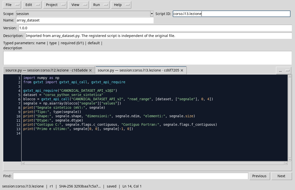
The code reads a variable of the Dataset and examines the structure.
Execution
- Open Session with
corso_python_serie_sinteticaand Viewer Python Scripts. - Import
dataset_arrays.py, assigns name and Script ID into thesessionbroom and saves. - Open Run → Open Script Runner…, run with Run Job and read the output.
- In the example shown, it controls the four values,
shape (4, 1),ndim 2,size 4anddtype float64. The first value is 1.2 mV and the last 1.6 mV.
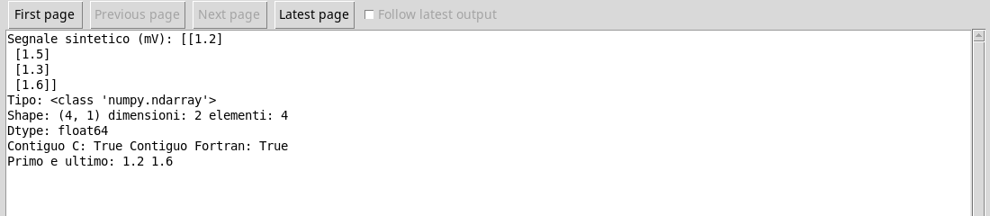
The observed array is a column of four synthetic values.
Common error
Use only one index such as signal[0] on a (4, 1) array selects a row, which can still be an array; signal[0, 0] selects the item. Do not automatically flatten the structure to run an operation: first check if the column axis has a meaning and if the operation requires a specific form.
Exercise
For an array with shape (3, 2), how many axes and elements are there? Which index selects the element of the third row and second column?
Worked solution
The axles are two and the elements are 3 × 2 = 6. The index is [2, 1], because both indexes start from zero. The form alone does not say which physical size represents each column: metadata is required.
In the next lesson we will select subintervals and columns maintaining the relationship between coordinates and values.