

Interpolation and Numerical Sampling
Scientific Python in GX-TXT · Module 5 · Lesson 26
A series of values can only be available at certain moments. Interpolation builds an estimate between those points according to a chosen model. In this lesson, we are playing a small synthetic curve with the linear method of the GX-TXT numerical API.
Objectives
- To build a grid of times and to distinguish the original knots from the points of question.
- Interpret linear interpolation and its validity at the edges.
- Call
NUMERIC_API_v1from the Runner and check the values obtained.
From grilled samples
Suppose we have (0 s, 0 mV), (1 s, 2 mV) and (2 s, 1 mV) points. We chose them for the exercise: they are not measures. We also want to estimate the signal to 0,5 s and 1,5 s. Linear interpolation connects each pair of next points with a segment. Half between 0 and 2 mV we get 1 mV; half between 2 and 1 mV we get 1.5 mV.
The grid is the set of ascisses that we ask for an estimate. np.linspace(0.0, 2.0, 5) produces five equidistant values, including both extremes: [0, 0.5, 1, 1.5, 2]. The order and monotony of the original ascisses are essential: a sequence with repeated times or out of order requires an explicit choice of preparation of the data before interpolation.
Run in GX-TXT
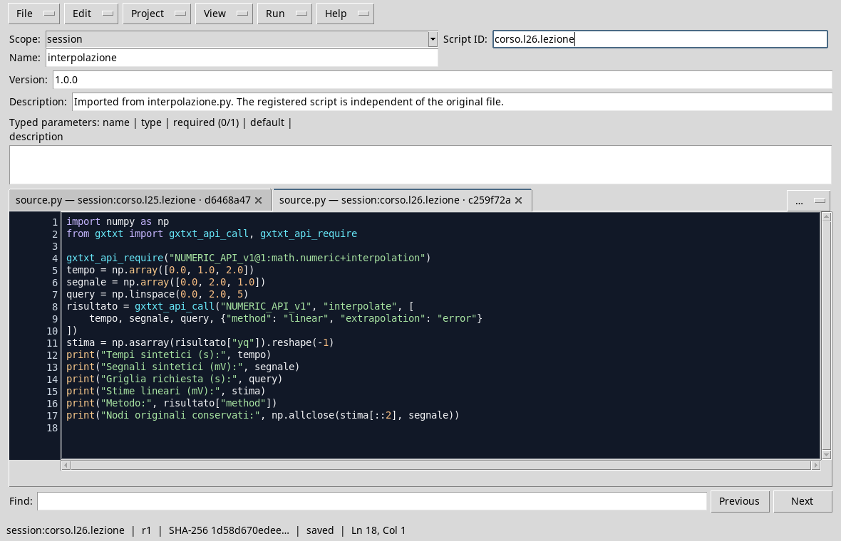
In the corso_python Session, import interpolation.py into the Python Script Workspace, save the script and run it from Run → Open Script Runner → Run Job.
import numpy as np
from gxtxt import gxtxt_api_call, gxtxt_api_require

gxtxt_api_require("NUMERIC_API_v1@1:math.numeric+interpolation")
time_values = np.array([0.0, 1.0, 2.0])
signal = np.array([0.0, 2.0, 1.0])
query = np.linspace(0.0, 2.0, 5)
result = gxtxt_api_call("NUMERIC_API_v1", "interpolate", [
    time_values, signal, query, {"method": "linear", "extrapolation": "error"}
])
estimate = np.asarray(result["yq"]).reshape(-1)
print("Synthetic times (s):", time_values)
print("Synthetic signals (mV):", signal)
print("Grid required (s):", query)
print("Linear estimates (mV):", estimate)
print("Metodo:", result["method"])
print("Original preserved nodes:", np.allclose(estimate[::2], signal))
gxtxt_api_require control requires interpolation capacity. The interpolate call receives the ascisses, orders, required points and a dictionary of options. method: linear chooses straight segments; extrapolation: error requires you to report a query outside the original range, instead of automatically inventing values beyond borders.
The answer contains yq, i.e. the estimated orders, and method information. np.asarray(...).reshape(-1) makes the result a NumPy flat carrier; estimate[::2] selects the elements to indexes 0, 2 and 4, which in this particular grid correspond to the original times. np.allclose verifies that estimates in those nodes coincide with the starting values within a numerical tolerance.
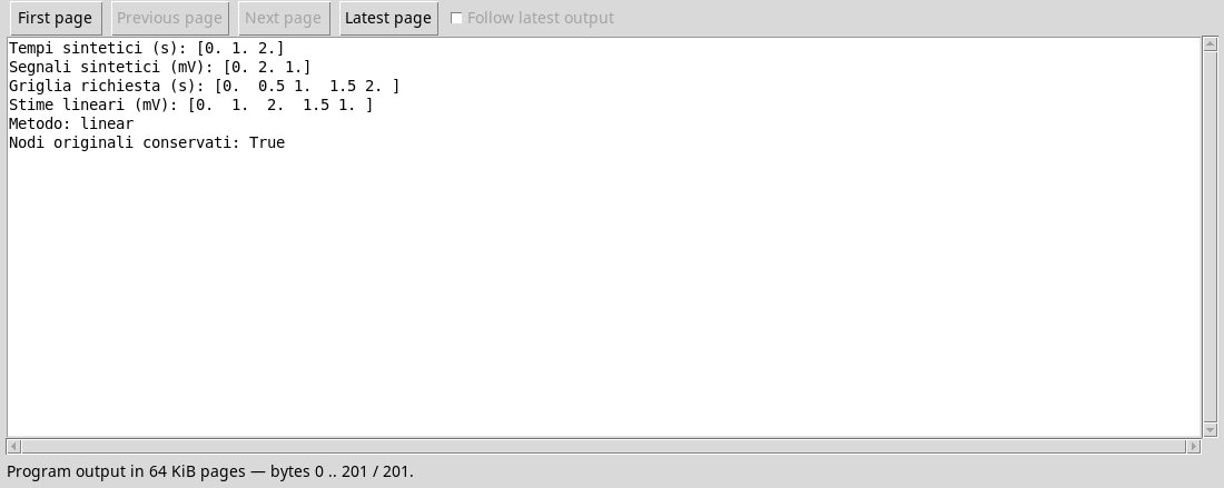
The result is [0, 1, 2, 1.5, 1] mV. The values at 0.5 and 1.5 s are produced by the linear model: they are not new measures. A good deal to the knots does not show that the real phenomenon follows straight segments between them. The choice of the method depends on the phenomenon, the density of the data and the presence of noise.
Interpolation and extrapolation
A request between the first and the last time is interpolation. A request, for example, at 2,5 s is extrapolation and requires assumptions about behavior beyond the available data. We chose the explicit refusal here. The API also documents other policies: adopt them only when they have meaning to the problem and describe them together with the results. If you save or publish the estimated series, it retains the distinction between source and derivation, method, grid and units.
Exercise
- Hand calculate the linear estimate to
0,25 s. What is unity? - Change the grid to get nine points between 0 and 2 s. What step do you get?
- If you ask for a value to
-0,5 s, why does the chosen option not allow you to treat it as an interpolated point?
Worked solution
- The first segment grows by 2 mV per second. At
0,25 sthe estimate is0,5 mV. - With
np.linspace(0.0, 2.0, 9)there are eight equal intervals, so the step is0,25 s. The indexes of the original knots change: for this grid are 0, 4 and 8. -0,5 sprecedes the first node: it is outside the domain of the series and would require extrapolation. Withextrapolation: errorthe request is rejected.
In the next lesson we will build a regression line and read the residues, without confuse a model that adapts to the data with a causal explanation.