

Linear Regression and Least Squares
Scientific Python in GX-TXT · Module 5 · Lesson 27
A straight can sum up an approximate relationship between two sizes. In this lesson we estimate intercept and slope with the GX-TXT numeric API and study what remains out of the model: the residues. All data are synthetic and adimensional.
Objectives
- Write the \(y=a+bx\) model.
- Understand the criterion of the minimum squares and the project matrix.
- Distinguish the expected values, residues and observations.
- Evaluate form, rank and conditioning before interpreting a fit.
The problem
We create five ascisses from 0 to 4 and a series according to \(y=1+2x+\varepsilon\). Noise is a specially chosen sequence, [0.1, -0.1, 0, -0.1, 0.1]: it does not represent an experiment or a measured statistical distribution. The resulting values are [1.1, 2.9, 5.0, 6.9, 9.1].
The ordinary linear regression chooses the parameters that minimize the sum of the squares of the residues, i.e. the differences observed - predicted. Raising to the square makes positive contributions and attaches more weight to the big differences. For these particular data, the noise has been chosen so that the optimal straight has intercepted 1 and slope 2, apart from small effects of the mobile comma.
Execution
In the corso_python Session, import regression.py, save the script in the Python Script Workspace and run it from Run → Open Script Runner → Run Job.
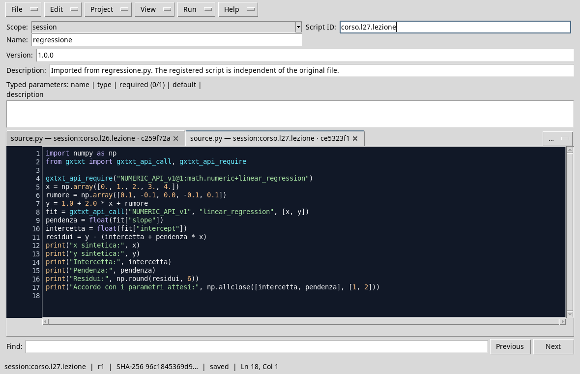
import numpy as np
from gxtxt import gxtxt_api_call, gxtxt_api_require

gxtxt_api_require("NUMERIC_API_v1@1:math.numeric+linear_regression")
x = np.array([0., 1., 2., 3., 4.])
noise = np.array([0.1, -0.1, 0.0, -0.1, 0.1])
y = 1.0 + 2.0 * x + noise
fit = gxtxt_api_call("NUMERIC_API_v1", "linear_regression", [x, y])
slope = float(fit["slope"])
intercept = float(fit["intercept"])
residuals = y - (intercept + slope * x)
print("x synthetic:", x)
print("Synthetic:", y)
print("Intercept:", intercept)
print("Pendence:", slope)
print("Residues:", np.round(residuals, 6))
print("Agreement with the expected parameters:", np.allclose([intercept, slope], [1, 2]))
The prior request identifies the ability to regression. The linear_regression call receives x and y; by default it includes the intercept and uses minimum standard weightless squares. The answer shows slope and intercept. The script calculates the forecasts with those parameters and removes each prediction from the corresponding synthetic value.
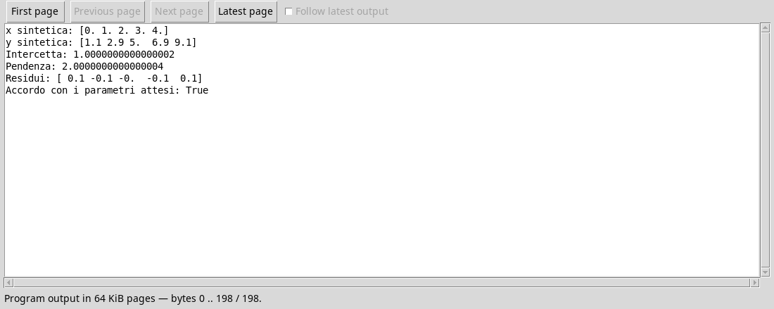
The output shows very close to 1 and 2. Small additional digits are normal effects of calculators in mobile commas; np.allclose uses tolerance. The residues coincide with the noise inserted, with numerical precision, because this example has been specially designed. With different data, the estimated parameters do not necessarily coincide with those used to generate data.
Project matrix and problem conditions
The model can be written as a product between a project matrix and the vector of parameters. Here each row of the matrix is [1, x_i], while the vector contains [intercept, slope]. The first column represents the constant term; the second associates every x value to the slope. Five observations for two parameters make the problem overdetermined: in general there is no straight that passes exactly for all points.
It is not enough to have more rows than columns. If all x were identical, the two columns would not be independent and the slope would not be uniquely identifiable. Even when the rank is complete, columns with very different scales can make the problem poorly conditioned: small changes in data can produce large variations of the parameters. Check rank, condition number and scale of variables; evaluate a centering or scale change consistent with the problem. The least_squares API allows an explicit project matrix and provides diagnostics, but requires you to comply with your contract.
If x and y had physical units, the intercept would have the y unit and the gradient of y divided for that of x. The goodness of a straight does not prove a causal relationship: they serve an experimental design and appropriate hypotheses. Weights, uncertainties and correlations also require an appropriate model; this example is an unweighted ordinary regression.
Exercise
- For \(x=3\), what value does the estimation and what residual result from the synthetic data?
- How many columns have the project matrix for a straight with intercept? Write the row corresponding to \(x=3\).
- Why does five observations with the same value of
xnot just identify separately intercept and slope?
Worked solution
- The forecast is \(1+2\cdot3=7\); the data is
6,9, so the less predicted residual is-0,1. - Two columns; the row is
[1, 3]. - The columns of the project matrix are proportional. Many pairs of parameters produce the same value in that only ascissa; the rank is not enough.
In the next lesson we will pass to non-linear models and Python functions used as callbacks.