

Functions as Objects and Nonlinear Fitting
Scientific Python in GX-TXT · Module 5 · Lesson 28
A non-linear model can describe a curve that is not a straight. In this lesson, we pass a Python function to the GX-TXT numeric API through a callback and draw the parameters of a synthetic exponential decay.
Objectives
- Use a Python function as a passable value to another operation.
- Record and release a callback for the Bridge.
- Perform a fit and control convergence and residues.
- Understand the role of the shape of the initial arrays and values.
The model
We consider \(y=A\exp(-kx)\), with A width and k decay constant. We create nine synthetic points with A = 3 and k = 0,7; we do not add noise to make the comparison immediately. The fit starts instead from [2, 0.5] and looks for parameters that reduce the differences between model and data.
The model is non-linear in the parameters: k appears in the exponent. The numerical solution also depends on the initial values, options and the shape of the problem. A solver can stop without converging or finding a result not suitable for scientific interpretation.
A function as a callback
In Python a function is an object: the name model can be passed without brackets, i.e. without performing it immediately. gxtxt_callback_register(model) records this function for current execution and returns a handle, a matte reference that we pass to Bridge. The solver can thus recall the function several times with different parameters.
The function must return a prediction for each observation. Here reshape(-1) makes parameters and ascisses monodimensional vectors; the NumPy formula produces a value for each ascissa. The callback must remain dedicated to the calculation and should not make nested Bridge calls: the call that activated the callback is still in progress.
Run the example
In the corso_python Session, import callback_fitting.py, save it in the Python Script Workspace and start it with Run → Open Script Runner → Run Job. The callback path of the provider uses SciPy in the Python runtime configured.
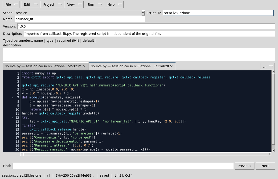
import numpy as np
from gxtxt import gxtxt_api_call, gxtxt_api_require, gxtxt_callback_register, gxtxt_callback_release

gxtxt_api_require("NUMERIC_API_v1@1:math.numeric+script_callback_functions")
x = np.linspace(0.0, 2.0, 9)
y = 3.0 * np.exp(-0.7 * x)
def model(parameters, x_values):
    p = np.asarray(parameters).reshape(-1)
    t = np.asarray(x_values).reshape(-1)
    return p[0] * np.exp(-p[1] * t)
handle = gxtxt_callback_register(model)
try:
    fit = gxtxt_api_call("NUMERIC_API_v1", "nonlinear_fit", [x, y, handle, [2.0, 0.5]])
finally:
    gxtxt_callback_release(handle)
parameters = np.asarray(fit["parameters"]).reshape(-1)
print("Convergence:", fit["converged"])
print("Range and decay:", parameters)
print("Expected parameters:", [3.0, 0.7])
print("Maximum residue:", np.max(np.abs(y - model(parameters, x))))
The try/finally block releases the handle even if the call to the fit raises an exception. After the release it should not be reused; the handle belongs to the current execution. The result preserves the numerical values of the fit. In this interface nonlinear_fit arguments are ascisses, observations, model handle and initial parameters.
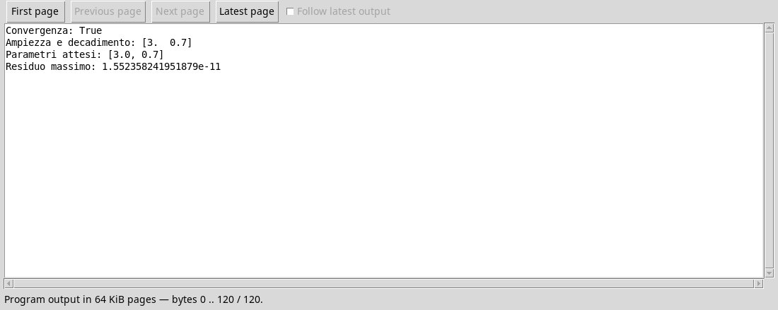
The provider reports converged: True; estimates are about [3, 0.7] and the maximum absolute residual is about 1,6 × 10⁻¹¹. The Job completed alone does not guarantee the convergence of the solver: the dedicated field must be read separately. The very small residue is consistent with data generated exactly by the same model, without noise; it does not guarantee the validity of the model on a real phenomenon.
def, lambda and closure
def is convenient for a function with multiple instructions and a clear name. A lambda can express a short function, such as lambda x: x * 2, but does not automatically improve readability. A closure is a function that uses defined values within which it surrounds it: it is useful to fix a constant, as long as it is clear what value is used. For the fit also consider the units: if x is in seconds, k is in s⁻¹; the argument of the exponential must be adimensional.
Exercise
- What values does the model provide for \(x=0\) and why?
- Why is it not enough to check that Job is completed?
- If the ascisse array has nine elements, how many values should the callback return?
Worked solution
- \(\exp(0)=1\), therefore the forecast is
A; in the example is 3. - The programme can normally end with a solver that signals lack of convergence. You have to read
convergedand interpret parameters and residuals. - Nine, one for observation. An incompatible form does not satisfy the contract of the model.
In the next lesson we will use callback to look for a zero and we will interpret the solver’s arrest condition.