

Differential Equations and ODE Callbacks
Scientific Python in GX-TXT · Module 5 · Lesson 30
An ordinary differential equation describes how a state changes compared to an independent variable, often time. In this lesson we integrate a synthetic decay into the GX-TXT Runner and compare the numerical values with a known analytical solution.
Objectives
- Interpreting derivatives, status and initial condition.
- Provide a Python callback with the derivative to the solver.
- Distinguish the times required by the internal steps of an adaptive method.
- Compare the numerical solution with a reference and read the error.
The model
We consider \(\frac{\mathrm{d}y}{\mathrm{d}t}=-0{.}7y\), with \(y(0)=3\). If time is in seconds, the 0,7 coefficient has s⁻¹ units. The analytical solution is \(y(t)=3\exp(-0{.}7t)\): starts from 3 and decreases over time. These are data and synthetic parameters chosen for the exercise.
The initial condition selects a specific solution between those compatible with the equation. The solver receives the derivative, the growing sequence of times and the initial state. An adaptive method internally chooses steps suitable for error criteria: the five times required for output should not be confused with all internal steps.
Run in GX-TXT
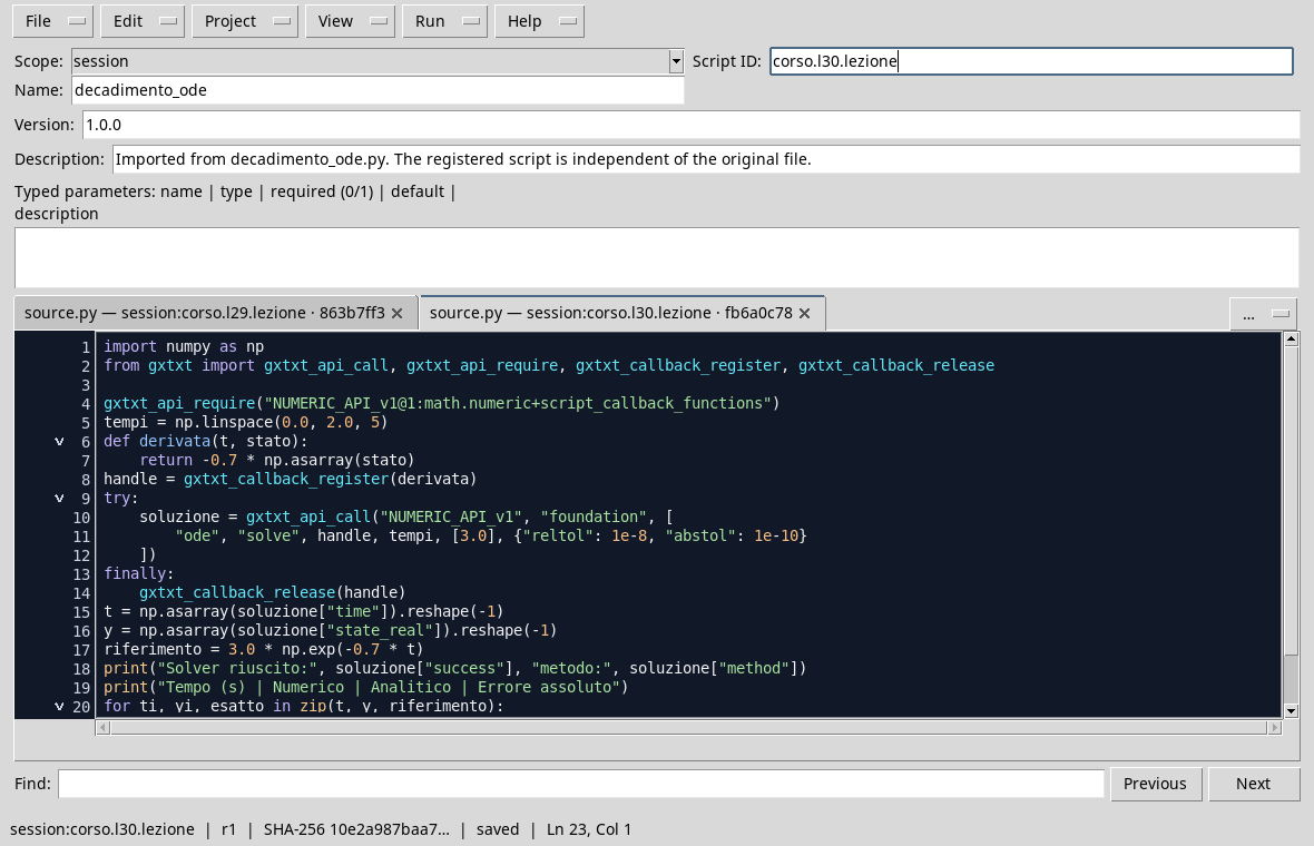
In the corso_python Session, import decay_ode.py, save it in the Python Script Workspace and start it with Run → Open Script Runner → Run Job. The callback path uses SciPy in the Python runtime configured.
import numpy as np
from gxtxt import gxtxt_api_call, gxtxt_api_require, gxtxt_callback_register, gxtxt_callback_release

gxtxt_api_require("NUMERIC_API_v1@1:math.numeric+script_callback_functions")
times = np.linspace(0.0, 2.0, 5)
def derivative(t, state):
    return -0.7 * np.asarray(state)
handle = gxtxt_callback_register(derivative)
try:
    solution = gxtxt_api_call("NUMERIC_API_v1", "foundation", [
        "ode", "solve", handle, times, [3.0], {"reltol": 1e-8, "abstol": 1e-10}
    ])
finally:
    gxtxt_callback_release(handle)
t = np.asarray(solution["time"]).reshape(-1)
y = np.asarray(solution["state_real"]).reshape(-1)
reference = 3.0 * np.exp(-0.7 * t)
print("Solver succeeded:", solution["success"], "metodo:", solution["method"])
print("Time (s) | Numeric | Analytical | Absolute Error")
for ti, yi, exact in zip(t, y, reference):
    print(f"{ti:5.2f} | {yi:9.6f} | {exact:9.6f} | {abs(yi-exact):.2e}")
print("Maximum error:", np.max(np.abs(y - reference)))
The derivative(t, state) function returns a derivative for each component of the state. We register the function and pass the handle to foundation, ode family, solve action. The finally lock also releases the handle in case of exception. Do not call the Bridge from the inside of the callback.
reltol and abstol set the relative and absolute tolerances used by the solver; choosing smaller values can increase the calculation work and does not alone guarantee the exactness of the model. The result shows the method and the successful state, the times and the numerical state. The analytical solution is evaluated at the same time to make comparison sensible.
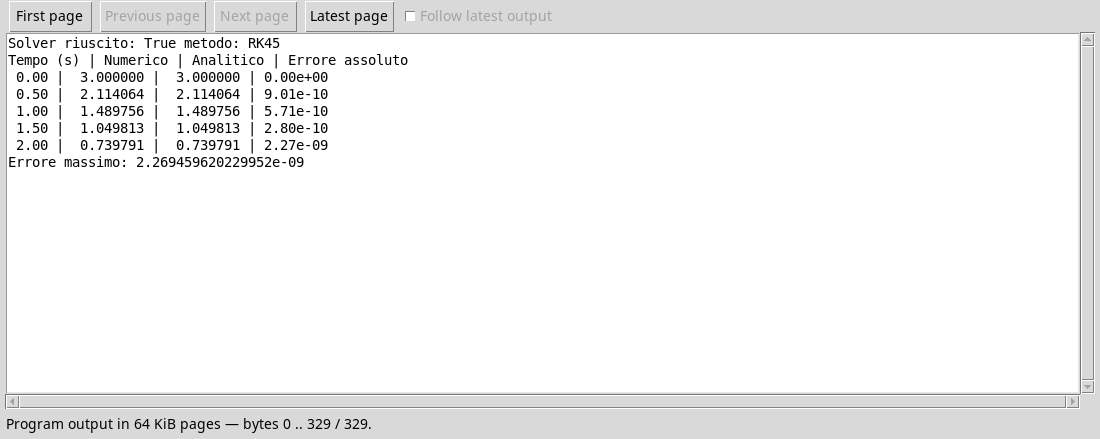
Here the method reported is RK45 and the solver signals success. The first value respects the initial condition; at the five times required the absolute maximum error compared to the formula is about \(2{.}3\times10^{-9}\). This value concerns the grid and the problem chosen: local tolerances and punctual comparison do not constitute a general guarantee of the overall error or the physical validity of the model.
View decay
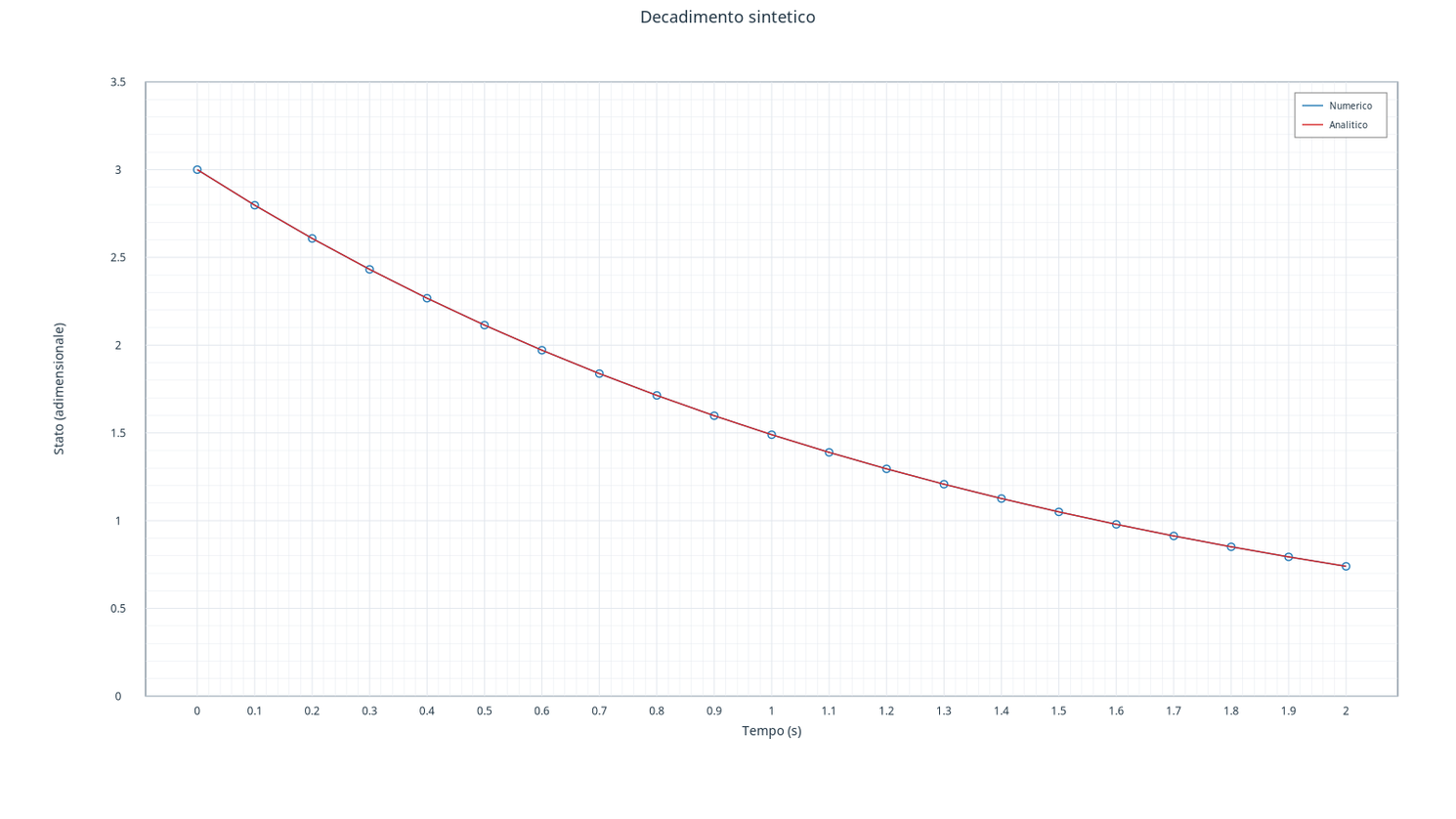
The additional script ode_plot.py integrates the same equation over 21 times, publishes separately the numerical and analytical solution and creates the graph with Plot API v4. In the GX-TXT graphics window, the curves are practically overlapped; the state is adimensional and the time is in seconds.
What to control in real problems
The units in the derivative must be consistent with those of the state and time. The grid of times must be strictly increasing for this interface. For systems with multiple components, callback returns a carrier of the same length of the state. A solver that does not complete integration does not automatically provide a reliable solution: you need to read the outcome and review model, conditions and parameters. In the next module we will learn how to represent data and results in the Viewer GX-TXT.
Exercise
- What value should
yhave in the initial time? What is the initial derivative? - What changes if the initial condition becomes 6, maintaining the same coefficient?
- Are the five times of output necessarily the only five steps of the solver?
Worked solution
- \(y(0)=3\); the derivative is \(-0{.}7\cdot3=-2{.}1\) state unit per second.
- The solution becomes \(6\exp(-0{.}7t)\): it doubles at any time, while the decay rate remains the same.
- No. RK45 adapts the internal steps; the specific grid where we want to receive the results.
Continue with the module on scientific visualization to build a chart from canonical data.