

Multiple Series, Styles and Legends
Scientific Python in GX-TXT · Module 6 · Lesson 34
A graph with multiple series allows to compare trends on the same reference system. In this lesson we publish a second synthetic series and show it together with the first, maintaining explicit identity and unity.
Objectives
- Compose a serial list in a PlotSpec.
- Connect each series to your Dataset and its variables.
- Distinguish curves by labels and legend.
- Interpret a comparison without confusing synthetic data and measures.
Preparation
The A series is in the corso_python_serie_sintetica Dataset. The script publishes the B series in the Dataset corso_python_seconda_serie, with [0, 0.5, 1, 1.5] s times and [1.0, 1.1, 1.2, 1.3] mV values. Both are built for the course: no one represents real observations.
In the corso_python Session, import multiple_series.py, save the script and run it from Run → Open Script Runner → Run Job.
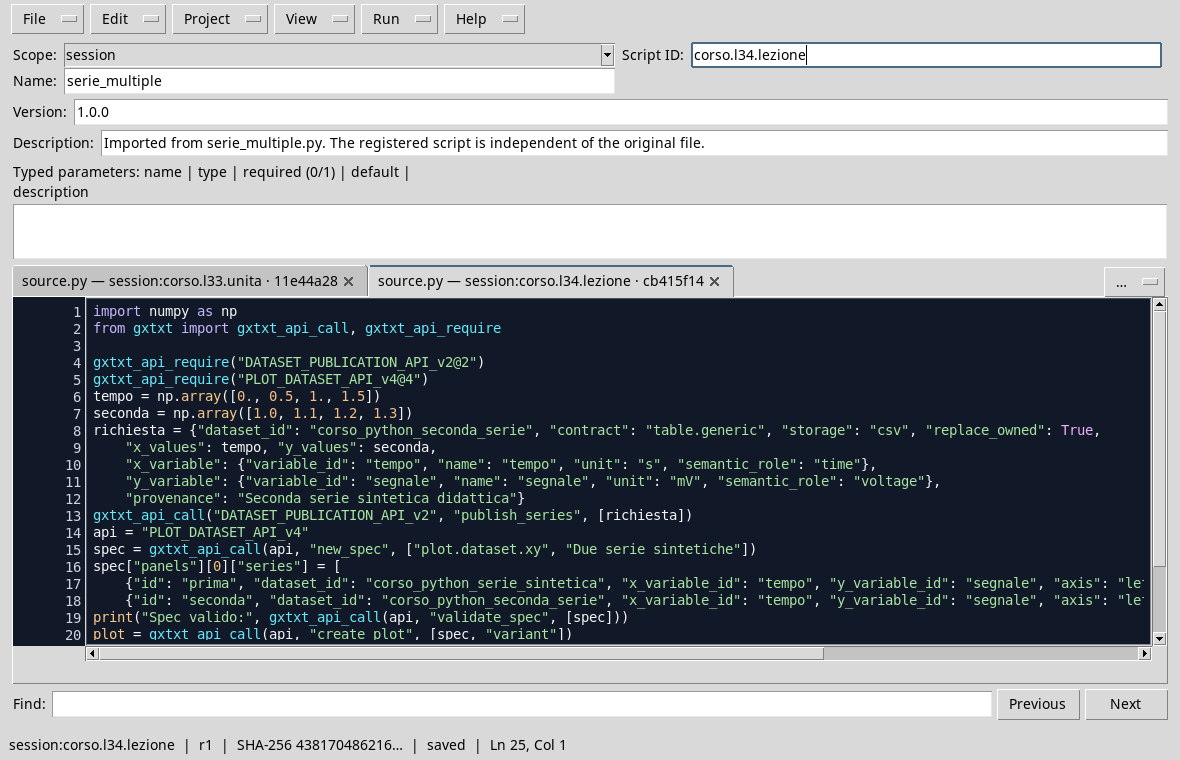
import numpy as np
from gxtxt import gxtxt_api_call, gxtxt_api_require

gxtxt_api_require("DATASET_PUBLICATION_API_v2@2")
gxtxt_api_require("PLOT_DATASET_API_v4@4")
time_values = np.array([0., 0.5, 1., 1.5])
second = np.array([1.0, 1.1, 1.2, 1.3])
request = {"dataset_id": "corso_python_seconda_serie", "contract": "table.generic", "storage": "csv", "replace_owned": True,
    "x_values": time_values, "y_values": second,
    "x_variable": {"variable_id": "tempo", "name": "tempo", "unit": "s", "semantic_role": "time"},
    "y_variable": {"variable_id": "segnale", "name": "segnale", "unit": "mV", "semantic_role": "voltage"},
    "provenance": "Second synthetic didactic series"}
gxtxt_api_call("DATASET_PUBLICATION_API_v2", "publish_series", [request])
api = "PLOT_DATASET_API_v4"
spec = gxtxt_api_call(api, "new_spec", ["plot.dataset.xy", "Two Synthetic Series"])
spec["panels"][0]["series"] = [
    {"id": "prima", "dataset_id": "corso_python_serie_sintetica", "x_variable_id": "tempo", "y_variable_id": "segnale", "axis": "left", "kind": "line_marker", "label": "Synthetic series A"},
    {"id": "seconda", "dataset_id": "corso_python_seconda_serie", "x_variable_id": "tempo", "y_variable_id": "segnale", "axis": "left", "kind": "line_marker", "label": "Synthetic series B"}]
print("Expenditure valid:", gxtxt_api_call(api, "validate_spec", [spec]))
plot = gxtxt_api_call(api, "create_plot", [spec, "variant"])
gxtxt_api_call(api, "set_panel_axis", [plot, "main", "x", {"label": "Tempo (s)", "display_unit": "s"}])
gxtxt_api_call(api, "set_panel_axis", [plot, "main", "y_left", {"label": "Segnale (mV)", "display_unit": "mV", "min": 0.0, "max": 2.0}])
print("Graph:", plot)
print("Rendering:", gxtxt_api_call(api, "render", [plot]).get("execution"))
The list assigned to series contains two dictionaries. Each dictionary has a serial ID, a Dataset and two variable IDs. The label field provides the text of the legend; kind: line_marker draws a line and points. The program uses the same Y axis because both variables are expressed in mV and are comparable in the example. The choice must be verified for each new Dataset.
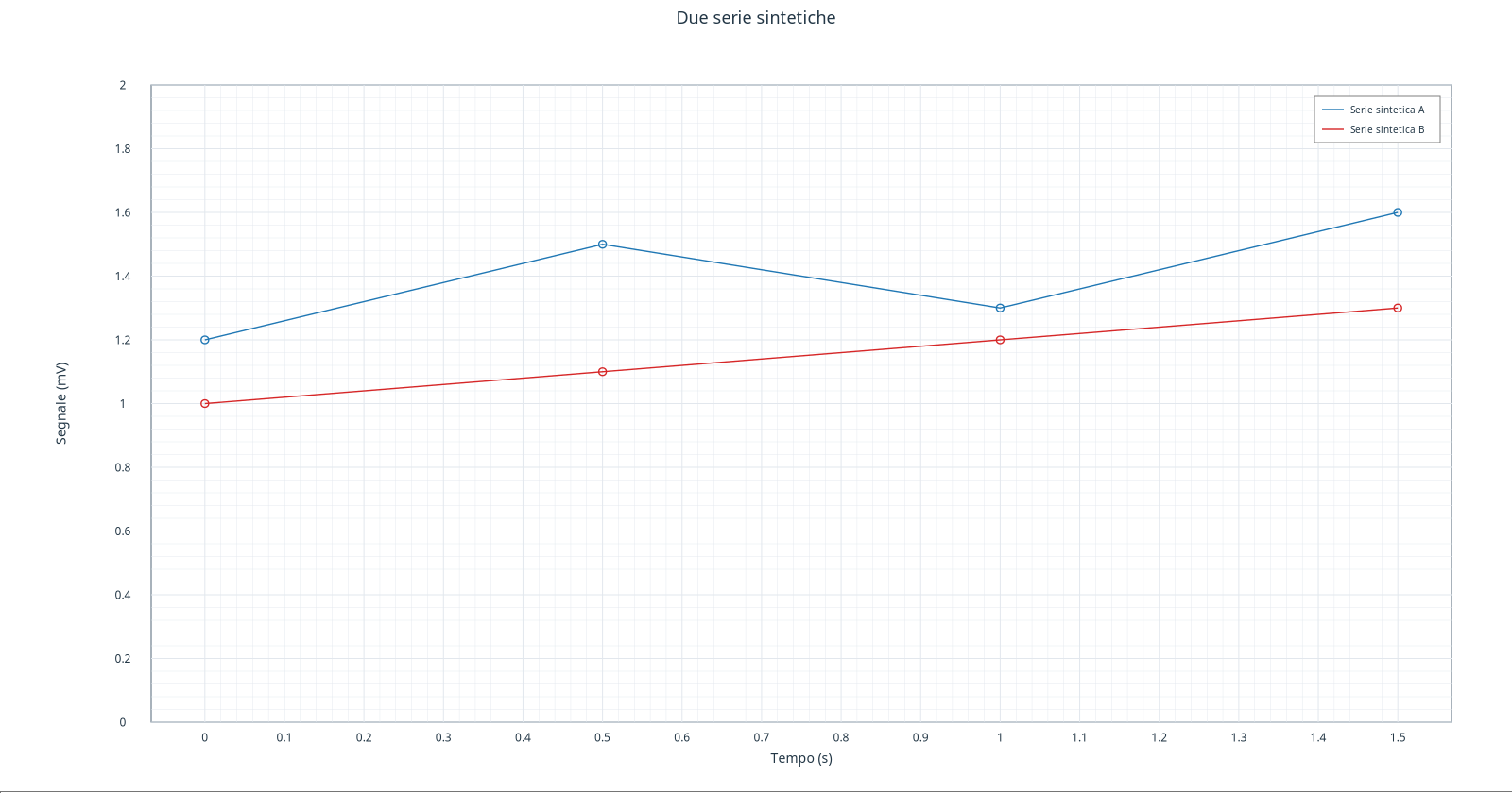
In this rendering the A series is blue and the B is red, with explicit labels. The colors are part of the presentation; the legend associates each track to its name. For graphs also intended for black and white printing or readers with difficulty in distinguishing colors, choose different dashes or markers when available, and check readability. Don’t just trust the color.
Read the comparison
At 0,5 s the A series is worth 1,5 mV and the B 1,1 mV. The difference is 0,4 mV at the points indicated. The graph does not say that a series is one measure and the other one prediction: both are synthetic. If it compares observations and models, declare it in the names and description, without attributing to estimates the status of measures.
Exercise
- What Dataset feed the two curves?
- What happens to the list
seriesif you add a valid third dictionary? - Why not just assign the same label to both series?
Worked solution
- Use
corso_python_serie_sintetica; B usecorso_python_seconda_serie. - The specification contains a third series: you need to assign unique IDs, valid references and a readable presentation.
- The legend would not allow to clearly distinguish the sources. Labels must identify what they represent.
In the next lesson we will separate the series in panels coordinated with a shared time axis.