

Multiple Panels and a Shared X-Axis
Scientific Python in GX-TXT · Module 6 · Lesson 35
When two series overlap or have different meanings, separate panels can make comparison clearer. Sharing the X axis allows you to compare the same moments without obliging variables to share the vertical axis.
Objectives
- Add a panel and assign it a series.
- Activate the multi-pannel layout and configure the shared X axis.
- Read the Y units and limits of each panel.
- Distinguish a layout choice from a data transformation.
Prepare the chart
The example uses the Synthetic Datasets of previous lessons: corso_python_serie_sintetica and corso_python_seconda_serie. Complete lesson 34 to publish the second Dataset. In the corso_python Session, import panels.py, save the script and run it from Run → Open Script Runner → Run Job.
from gxtxt import gxtxt_api_call, gxtxt_api_require

gxtxt_api_require("PLOT_DATASET_API_v4@4")
api = "PLOT_DATASET_API_v4"
spec = gxtxt_api_call(api, "new_spec", ["plot.dataset.xy", "Two synthetic signalals"])
spec["panels"][0]["series"] = [{"id": "prima", "dataset_id": "corso_python_serie_sintetica", "x_variable_id": "tempo", "y_variable_id": "segnale", "axis": "left", "kind": "line_marker", "label": "Series A"}]
plot = gxtxt_api_call(api, "create_plot", [spec, "variant"])
gxtxt_api_call(api, "add_panel", [plot, "secondo"])
gxtxt_api_call(api, "set_multi_panel", [plot, 1])
spec = gxtxt_api_call(api, "load_spec", [plot])
spec["panels"][1]["series"] = [{"id": "seconda", "dataset_id": "corso_python_seconda_serie", "x_variable_id": "tempo", "y_variable_id": "segnale", "axis": "left", "kind": "line_marker", "label": "Series B"}]
gxtxt_api_call(api, "apply_spec", [plot, spec])
gxtxt_api_call(api, "set_panel_title", [plot, "main", "Series A"])
gxtxt_api_call(api, "set_panel_title", [plot, "secondo", "Synthetic B series"])
gxtxt_api_call(api, "set_panel_axis", [plot, "main", "y_left", {"label": "A (mV)", "min": 0., "max": 2.}])
gxtxt_api_call(api, "set_panel_axis", [plot, "secondo", "y_left", {"label": "B (mV)", "min": 0., "max": 2.}])
gxtxt_api_call(api, "shared_x_axis_set", [plot, {"display_unit": "s", "scale": "linear"}])
print("Pannelli:", gxtxt_api_call(api, "panel_ids", [plot]))
print("Graph:", plot)
print("Rendering:", gxtxt_api_call(api, "render", [plot]).get("execution"))
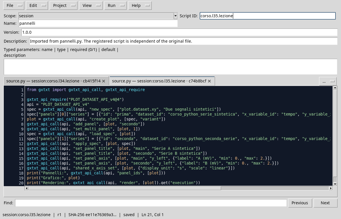
After creating the first variant, add_panel adds the secondo and set_multi_panel panel to activate the layout. load_spec reads the specification; we add the B series to the second panel and apply the new structure with apply_spec. Titles clarify what data are shown. Each Y axis has its own label and limits; here we have chosen 0–2 mV range to facilitate comparison.
shared_x_axis_set sets the scale and unit of the shared axis. The two time variables must be compatible: the fact that two columns are called both time_values is not enough alone to prove it. In this example they are both in seconds and describe the same synthetic grid.
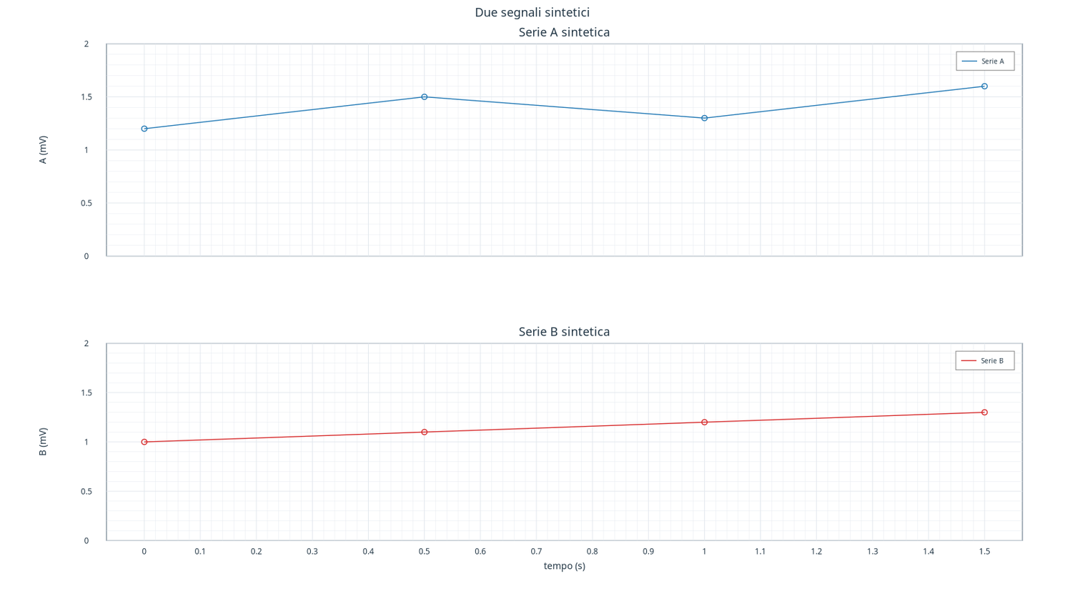
At 1 s, the 1,3 mV and the B 1,2 mV. The tracks are separated, but the horizontal positions correspond to the same times. The shared X axis coordinates reading: it does not heat or arbitrarily convert the ordered. If the panels represent different sizes, each must retain its own unit and a justified scale.
Exercise
- Which panel contains the B series?
- If you change the Y limit of the second panel, did you change the dataset values?
- What control is needed before sharing the time axis of two Datasets?
Worked solution
- The
secondopanel, displayed under the first. - No, you changed the presentation. However, the change can affect the perception of variations.
- Check that the coordinates represent the same magnitude and have compatible units, as well as checking their temporal meaning.
In the next lesson we will add textual information to the chart distinguishing annotation and data.