

Descriptive Statistics with Numerical APIs
Scientific Python in GX-TXT · Module 8 · Lesson 43
The descriptive statistics sum up a set of values. In this lesson we compare the results of the GX-TXT numerical API with NumPy for a synthetic series of four values in millivolt.
Objectives
- Calculate median and quantum.
- Distinguish variance of population and sample.
- Recognize the units of variance and standard deviation.
- Interpret a summary without giving independence to data.
Synthetic
We use [1.2, 1.5, 1.3, 1.6] mV. The average is the sum divided by four, 1,4 mV. By ordering the values we obtain [1.2, 1.3, 1.5, 1.6]: the median is the average of the two central values, also 1,4 mV. This equality is particular to the data chosen.
Execution
At the corso_python Session, import descriptive_statistics.py, save it and start it in the Runner.
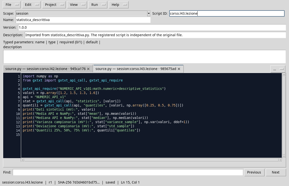
import numpy as np
from gxtxt import gxtxt_api_call, gxtxt_api_require

gxtxt_api_require("NUMERIC_API_v1@1:math.numeric+descriptive_statistics")
values = np.array([1.2, 1.5, 1.3, 1.6])
api = "NUMERIC_API_v1"
stat = gxtxt_api_call(api, "statistics", [values])
quantiles = gxtxt_api_call(api, "quantiles", [values, np.array([0.25, 0.5, 0.75])])
print("Synthetic data (mV):", values)
print("Media API and NumPy:", stat["mean"], np.mean(values))
print("Mediana API and NumPy:", stat["median"], np.median(values))
print("Sample variation (mV2):", stat["variance_sample"], np.var(values, ddof=1))
print("Field deviation (mV):", stat["std_sample"])
print("Quantities 25%, 50%, 75% (mV):", quantiles["quantiles"])
statistics returns a summary; quantiles calculates the quantities required. The sample variance uses the \(n-1\) divider: to compare it with NumPy we impose ddof=1. Population variance uses n instead. The choice depends on the quantity you intend to describe, not on which result you seem more convenient.
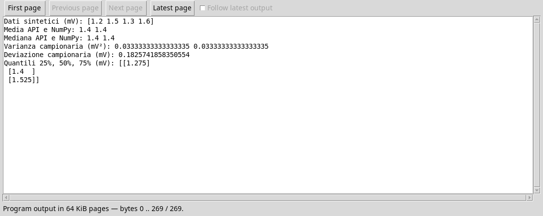
The sample variance is about \(0{.}0333\,\mathrm{mV}^{2}\) and the standard sample deviation about 0,1826 mV. The variance has units per square, while the standard deviation has the same data unit. The quarters shown use the type 7 definition of the API: about 1,275, 1.4 and 1,525 mV. Different methods of quantum can give different results, especially on small samples; declares the convention used.
Interpretation
Four values allow to calculate a summary, but do not show that the observations are independent or representative. In a time series neighboring values can be related. Media and dispersion do not describe by themselves the form of distribution, temporal trend or measurement uncertainty. Here the numbers are synthetic, not experimental observations.
Exercise
- What is the average of the series and in which unit?
- Why is variance expressed in mV2?
- What changes between
np.var(values)andnp.var(values, ddof=1)?
Worked solution
1,4 mV.- Variance measures the average squared deviation from the mean.
- The first uses the
ndivider; the second uses \(n-1\), corresponding to the sample variance of the example.
In the next lesson we will introduce weights and propagation of uncertainties.