

Sources and sampling
Select the Dataset and variables
- Scientific Dataset
- Open the selector and choose a canonical table of the Session. A file on the disk must first be imported. For exercises use the ZIP package that keeps IDs, units, and numeric types. When you change Dataset, check the three choices below.
- Primary measured signal
- Active and single-dimensional numerical variable to be analyzed. For FRF is the reference input.
- Paired signal (only when required)
- The second variable in the same Dataset. A distinct second channel is required only for
correlation.cross,spectral.coherence, and the two FRFs. Align the channels sample by sample on the same time base. For a frequency response, select the output channel here. For single-channel methods, leave this field blank. The field remains visible and a leftover selection may still be read and validated. - Measured time coordinate
- A numeric variable with a unit convertible to seconds, such as
ms. The chart shows the original unit, which the analysis converts to seconds. For an already normalized elapsed-time coordinate, the service uses that scale directly. - Scientific question / method
- Select one of the fifteen IDs. The default is
quality.basic. The viewer shows the applicable fields and in the report lists the provider’s internal field names. For their use, see chapters by family. - Reset
- The Reset button next to a field restores its default. For the primary signal, paired signal, and time coordinate, it clears the selection. For the method, it restores
quality.basic. Method-specific fields are hidden when irrelevant. Before switching methods, correct or reset out-of-range values. The request also validates numeric settings that the viewer retains.
Set the sampling rate
Use one of the two procedures.
- Measured time. Select Measured time coordinate and leave Declared sample rate [Hz]; 0 = use time axis at
0. The service converts the coordinate to seconds and estimates the interval as (last−first)/(N−1). Values must increase and stay within 10−6 times the interval of the uniform grid. The sample rate is the reciprocal of the interval. Thetime_msexample starts at 125 ms and yields 256 Hz. - Declared sample rate. Empty the coordinate with its Reset and write a positive frequency in Hz, for example
256. In time results the base starts from 0 s. The stated rate enables the calculation but for Display source you also have to choose an explicit coordinate.
If you supply both sources of timing information, the declared and measured rates must agree within a relative difference of 10−6. The report sets sampling to measured, declared, or unavailable. Quality metrics, correlations, envelope, and phase can work without a known rate. Spectral methods, instantaneous frequency, filtering, and decimation require one. Reset sets the declared rate back to 0.
Load and navigate the source plot
Select a time coordinate and a primary signal, then select Display source. The plot previews one channel. The backend may reduce the displayed point count using level of detail (LOD), with a display budget of 4,096 points. Fit and zoom change the viewport. The computation reads every selected row. In the dense test, the preview showed about 3,836 points while Analyze read all 20,000 rows.
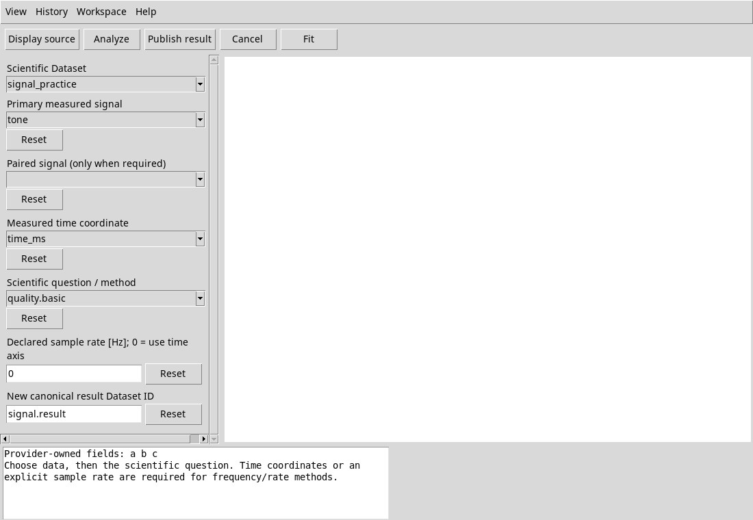
In the tested version, Display source can bind the source while the canvas stays blank, even after Fit. The calculation still works. To see the processed curve, publish the result and render the Plot v4 variant from the main window, as described in the publication procedure.
Use View → Fit, Fit in the bar or double-click to adjust the curve. Drag with the central button to translate the view. The left click is a point selection gesture when the curve is drawn. The fault of the canvas prevents the visual selection in this version. The viewer does not display a graphic context menu on this preview.
In the tested version, Zoom in widens the displayed range and Zoom out narrows it. Scrolling the wheel forward also widens the range. To zoom closer, use Zoom out. To restore the initial view, use Fit. These controls do not change sampling or results.
Input conditions that stop an analysis
At least three rows are required. The service rejects voltage units where time is required, descending or nonuniform axes, inconsistent sample rates, and integers too large for exact conversion. It rejects incomplete or nonfinite series without filling missing values. For integer data, the provider rejects magnitudes greater than 253. For a failed Job, review the log to identify the cause.
The service has a managed input budget of 2 GiB, counted as 8 bytes per row per distinct variable read. Exceeding the budget rejects the request. The old limit of 16,384 rows does not apply in this version. The 20,000-row test returned the full count.