Bind Data and Units
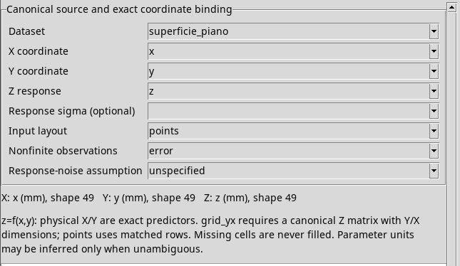
Canonical source and exact coordinate binding
In Dataset, choose the canonical ID of a source in the Session. The selector lists available IDs when the viewer opens. If a newly acquired source is missing, save any edits and reopen the viewer. Changing the Dataset reloads the variable lists. A variable that does not exist in the new source is cleared.
If you click Preview fit before assigning all three roles, the status line shows Choose canonical X, Y and Z Variables. Check that the Dataset is imported and contains the required variables.
- X coordinate
- Select the physical coordinate represented by
xin the expression. The selector lists eligible numeric vectors. - Y coordinate
- Select the physical coordinate represented by
y. The selector lists eligible numeric vectors. In a grid, the Y axis must use a different canonical dimension from X. - Z response
- Select the response to fit. The selector lists eligible numeric vectors and matrices. Use a vector in points and a matrix in grid_yx.
- Summary of variables
- In the text below the fields, check the ID, unit and shape. Each variable supports up to 65,536 source values. If the status reports a higher count, select a scientifically appropriate subset and save it as a canonical Dataset before retrying. The model uses the Dataset unit.
- Response sigma (optional)
- Leave this blank to fit without sigma values. If you have standard deviations for Z, select that variable. It must match Z in unit, shape, rank and canonical dimension IDs. Retained sigma values must be finite and strictly positive. Zero and negative values do not automatically exclude observations.
Input layout
- points
- This is the default layout. Use it for
(x,y,z)tuples in matching rows, such as an irregular point cloud. The three variables must share both the canonical row dimension and the row count. The original order and repeated observations are retained. - grid_yx
- Use this for X and Y vectors on distinct dimensions and a Z matrix ordered exactly as Y, X. Axis coordinates must be finite and unique. For five X values and four Y values, Z must have shape
4;5. Validation checks canonical dimension IDs as well. Usingsuperficie_grigliaand the calibration plane expression gives 20 observations and slopes close to 2.0025 and −0.70125. If you see Surface grid Z must have the exact ordered Y/X axis dimensions, correct the source Dataset before retrying.
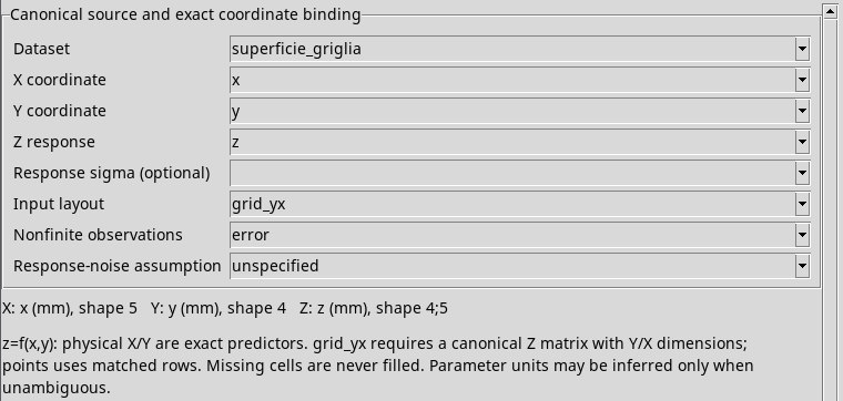
superficie_griglia contiene 20 risultati disposti su una matrice Y/X.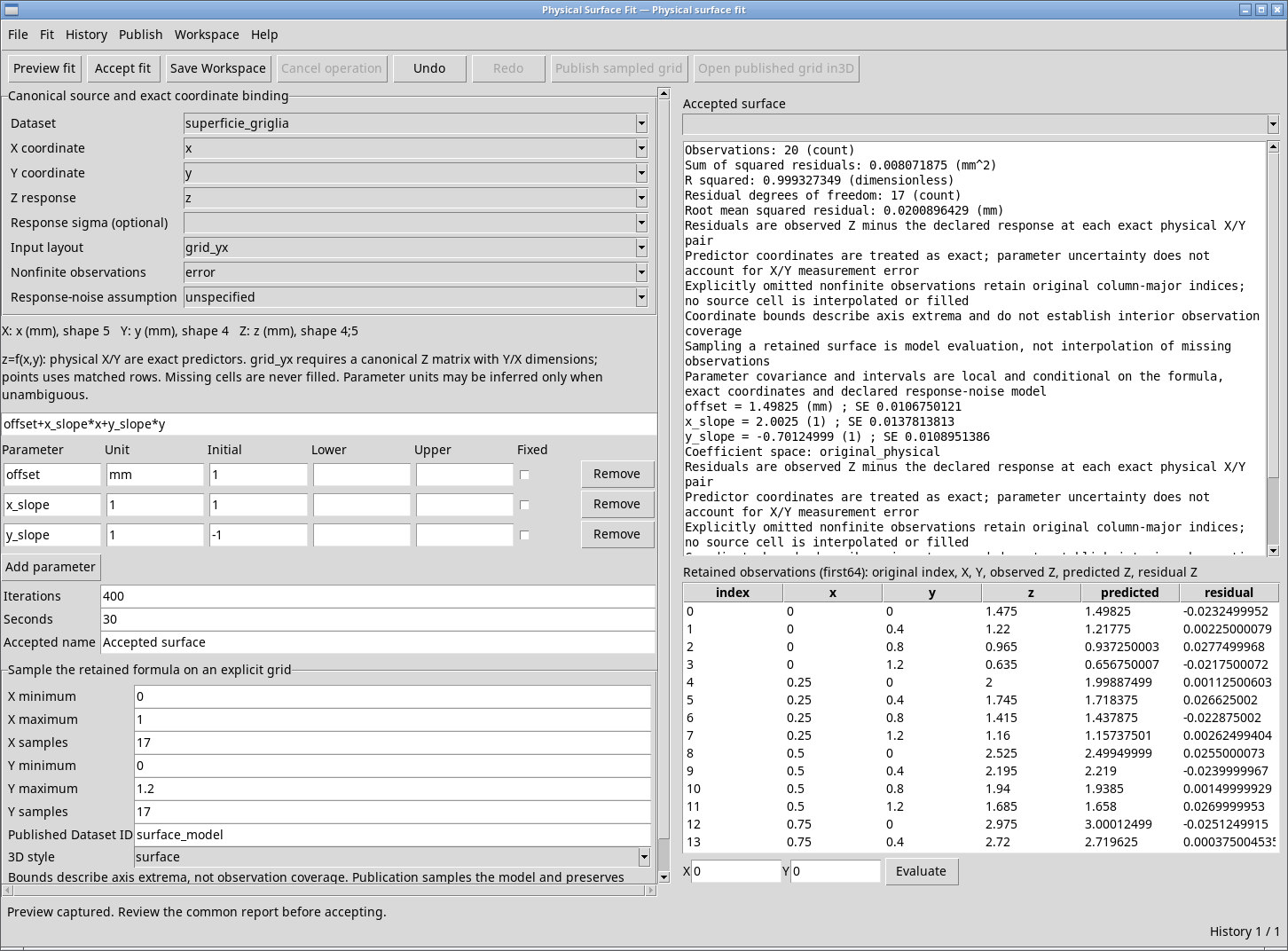
Nonfinite observations
- error
- This is the default policy. It rejects nonfinite observations. Use it first when checking for incomplete data.
- omit
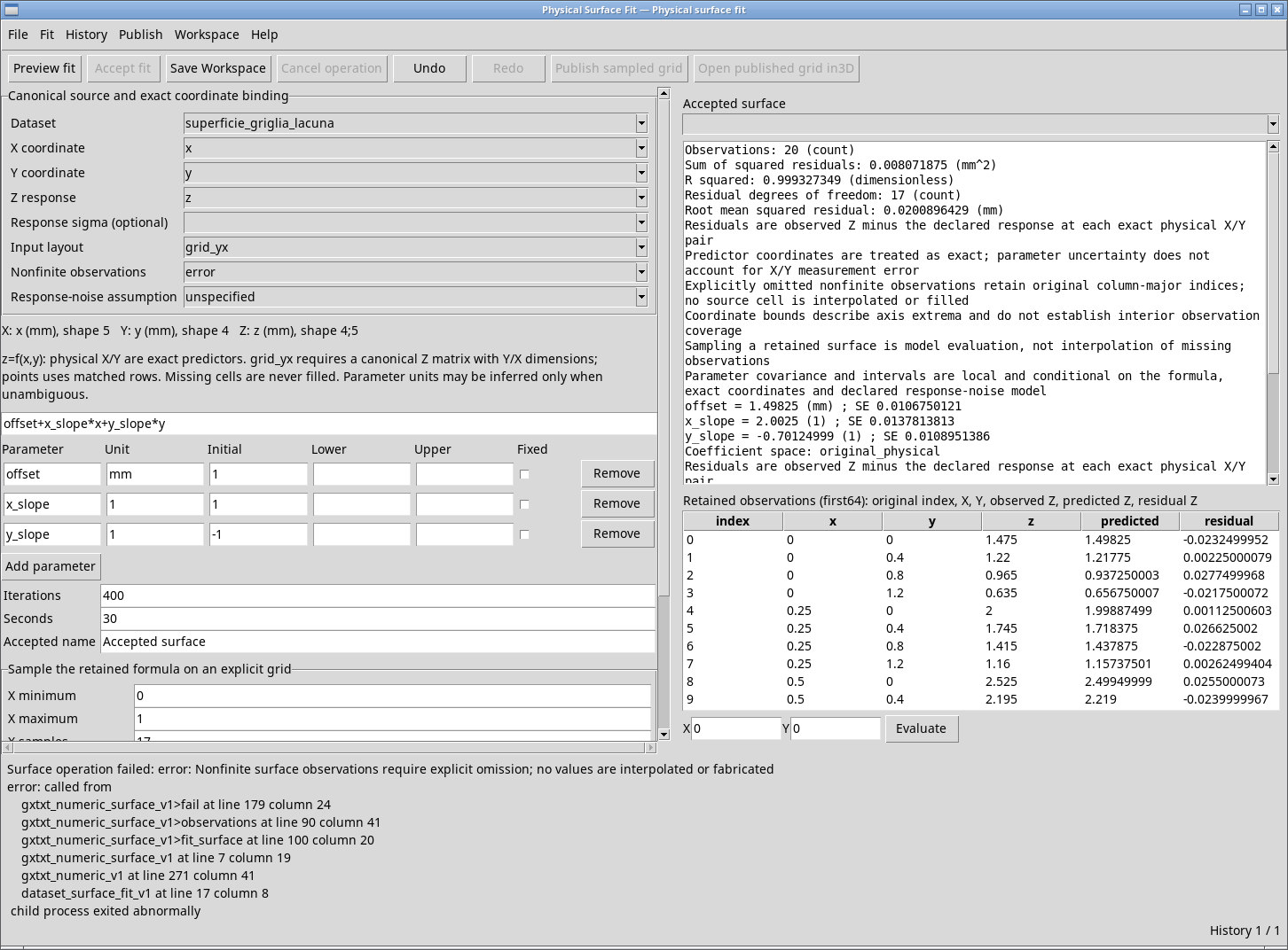
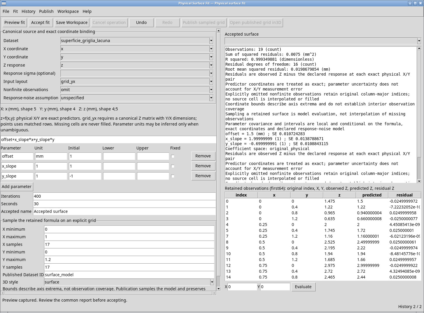
- Use this when the analysis should use only finite observations. Check the count and original indices in the table. On a grid with four Y values, Y index 2 in X column 1 corresponds to zero-based index
2 + 4 × 1 = 6. Withsuperficie_griglia_lacuna, switching policies yields 19 observations, with index 6 omitted. Withsuperficie_punti_lacuna, the fit uses 48 rows and preserves their original indices out of 49. A nonfinite grid axis in grid_yx requires a corrected source.
Response-noise assumption
- unspecified
- This default makes no Gaussian assumption. You can leave sigma blank or supply it to specify response uncertainty. Check the qualification and availability of each statistic in the report.
- independent_gaussian_known_sigma
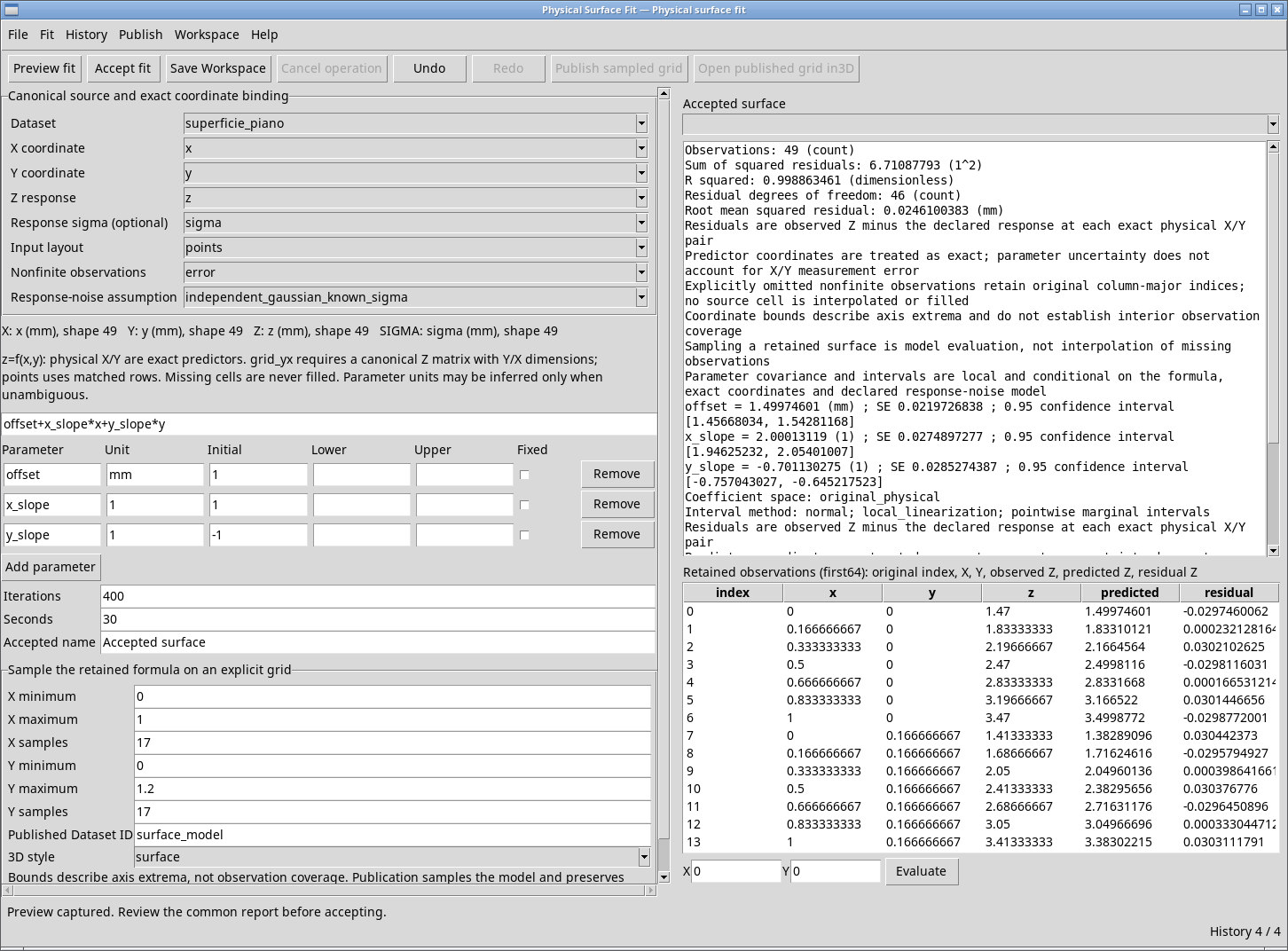
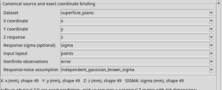
- Use this when response errors are independent and Gaussian with known sigma for each observation. Bind a compatible numeric variable in Response sigma (optional). For example, select
sigmain thesuperficie_pianoDataset. A sigma variable of a different shape or with nonpositive values is rejected. - independent_gaussian_estimated_variance
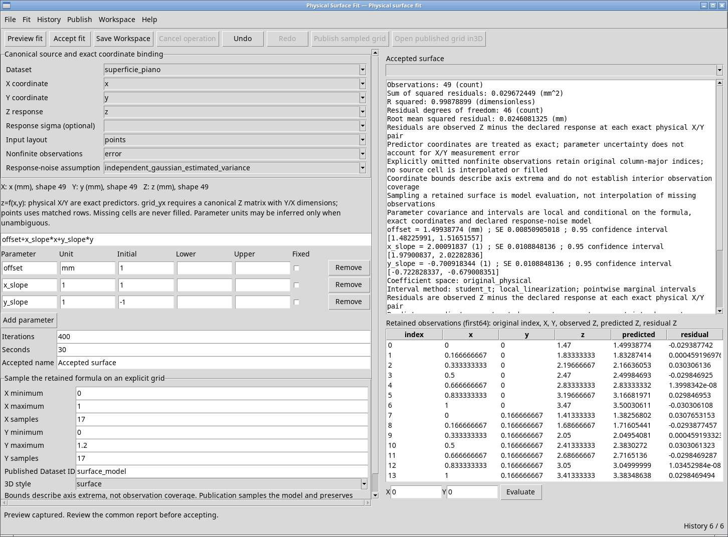
- Use this when response errors are independent and Gaussian with a common variance to be estimated. Leave Response sigma (optional) blank. If sigma is set, the viewer reports a conflict. Check the residual degrees of freedom before interpreting the estimates.
sigma.