

Evaluate and Accept the Fit
Calculate and review a preview
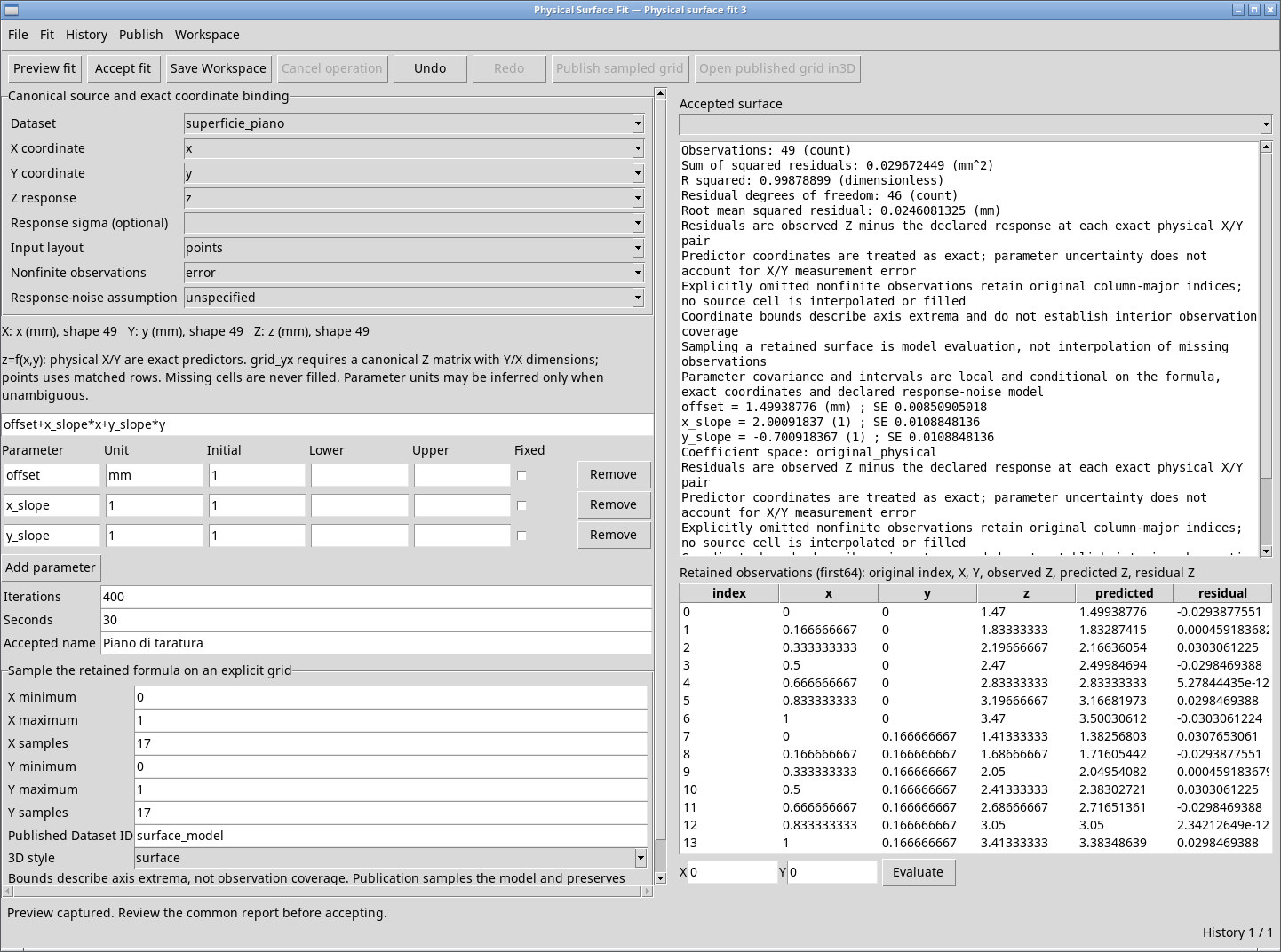
Bind the variables, define the expression and choose Fit → Preview fit or the corresponding button. You can also press F5 in the active window. While the fit is running, the status line indicates that computation has started and editing and saving are disabled. A successful calculation shows Preview captured. Review the common report before accepting. and adds an entry to History.

Fit → Cancel operation, its toolbar button and Esc interrupt the running operation. Surface operation cancelled confirms cancellation. Previously accepted fits remain available. The cancel command is disabled again when the operation ends.

If a run fails, read the status line. The previous report and residuals may still be visible. Correct the reported problem and run a fresh preview before interpreting the current draft.
Interpret the report
- Observations (n)
- Number of observations used. With omit, compare it with the original count to find how many observations were excluded.
- Sum of squared residuals (SSE)
- Sum of squared response residuals, in squared Z units. Coefficient estimation may use weights derived from the declared sigma values.
- R squared (R²)
- Compares the model’s squared residuals with the spread of Z about its mean. Use it as a descriptive check and inspect the residuals. It may be unavailable for a constant response.
- Residual degrees of freedom (dof)
- Residual degrees of freedom depend on the observations and free fit parameters. The report identifies locked parameters as fixed.
- Root mean squared residual (RMSE)
- Square root of the mean squared residual. It has the same unit as Z, so you can compare the calibration plane’s 0.0246 mm with measurement precision.
- Parameter estimates
- Each row gives the estimate and declared or inferred unit. Read the associated note. With unspecified, the viewer may show SE (a local standard error) without a confidence interval. Under Gaussian assumptions, the standard error and 95% interval appear when available. A fixed parameter retains its imposed value.
Read the residual table
The pane shows up to the first 64 retained observations. index is the original zero-based index. x and y are the source coordinates, z is the measured response, predicted is the modeled value and residual is z − predicted. For a grid, the index runs along Y within each X column. Gaps in the indices are expected with omit. A positive residual means the observation is above the modeled value.
Save and select a surface
After checking status, coefficients and residuals, enter Accepted name and choose Fit → Accept fit, the corresponding button or F6. The default name is Accepted surface. The status Accepted physical surface saved. confirms that the fit was saved and selected in Accepted surface. You can now evaluate Z, export the model or configure a grid. Use a recognizable name to distinguish fits in the same Workspace.
If you change the source, expression, parameters or solver limits after the preview, run Preview fit again. In this release, Accept fit can still look enabled even when it has no effect. You can change only the result name immediately before acceptance without running another preview.
Accepted surface is the selector above the report. When several fits are available, choose the one to inspect. The calibration plane gives 1.879204 mm at X = 0.4 mm and Y = 0.6 mm. A refit with the offset fixed at 1.5 mm gives about 1.879315 mm at the same coordinates. The report, residual table, evaluation, export and sampling all use the selected fit.
Evaluate at exact X and Y coordinates
- Accept and select a fit first. Without a result, Fit → Evaluate exact XY pair is disabled. Evaluate may look active, but clicking it leaves the state unchanged until you select an accepted fit.
- In the bottom-right pane, enter X and Y in the original variable units. Both fields start at 0. Enter finite numbers with a decimal point, such as
0.4and0.6in mm. - Click Evaluate or choose Fit → Evaluate exact XY pair. Read Z = … at exact X/Y; no refit. on the status line. The example plane gives about 1.879204 mm. The model evaluates the expression at the requested coordinates, including between sample points, with the existing coefficients.
Integers outside the consecutive exact-integer range of binary64, beyond ±9,007,199,254,740,992, are rejected. Both coordinates must stay within the fit’s retained bounds. If the input is rejected, check the units and retry within the original bounds. Bounds and observations describe the measured domain. A point inside that rectangle may still lie in a sparsely sampled region.
