Sample, Visualize and Export
Set up a model grid
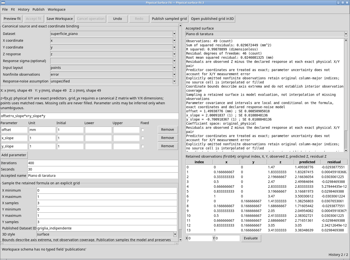
Select an accepted surface. Scroll down on the left to Sample the retained formula on an explicit grid. The grid holds the modeled values at the specified XY nodes. The source measurements and any missing cells remain intact.
- X minimum
- Lower bound in X units. If the field is blank when the first result appears, it takes the fit’s minimum X. Choose a value within the retained domain.
- X maximum
- Inclusive upper bound in X units. It starts at the fit’s maximum X and must exceed X minimum.
- X samples
- Number of equally spaced nodes, from 2 to 256 inclusive. The default is 17. Both bounds are included.
- Y minimum
- Lower bound in Y units, initially the fit’s minimum Y. It can narrow the sampled domain.
- Y maximum
- Inclusive upper bound in Y units. It starts at the fit’s maximum Y and must exceed Y minimum.
- Y samples
- Number of Y nodes, from 2 to 256, initially 17. Set it independently of X.
- Published Dataset ID
- Grid identifier within the Session. The default is
surface_model. Enter a valid, unused ID such asguida_piano_griglia. If the ID is already in use, enter a different one.
If you switch fits, recheck the bounds. Use finite numbers and integer sample counts. Grid axes require2..256 explicit samples signals a count outside the supported range. Grid upper bound must exceed lower bound signals equal or reversed bounds. A coordinate outside the fit domain is rejected.
Publish and verify the sampled Dataset
Choose Publish → Publish sampled grid or click the corresponding button. With five X nodes and four Y nodes, X has five values, Y has four, and Z is a 4 × 5 matrix in Y/X order. The canonical variables are named x, y and z and retain their original units.
In this release, Workspace schema has no typed field ‘publications’ may appear after the Dataset is created. Look for the ID in the Dataset browser before retrying. The Dataset can exist even if the fit-to-grid association failed. Publishing again with the same ID causes a conflict. The accepted model still supports Evaluate and export.
Open a published grid in 3D
In 3D style, surface is the default and requests a surface plot. mesh requests a wireframe. This setting changes how the grid is drawn. Grid values remain the same.
Select the accepted result and enter the ID of its unmodified published Dataset in Published Dataset ID. Use Publish → Open published grid in3D or click its toolbar button. If publication ended with the association error described above, both styles are rejected with Choose an unchanged canonical grid published from this accepted surface and the viewer does not open. In 3D Studio, Add Dataset 3D layer is intended for points or trajectories from a canonical CSV Dataset. It rejects the HDF5 grid produced in this workflow.

Export the function and metadata
Select the fit, choose File → Export model… and pick a folder with none of the four files listed below. If a file already exists, the status Export exists: identifies the one blocking the operation. Python, Octave, LaTeX and physical model metadata exported. confirms export. Close the folder picker with Cancel to return to the model.

fit_surface.py- Python function for XY pairs in the declared units. With NumPy installed, import
fit_surfaceand runfit_surface([[0.4, 0.6]]). Each returned row contains X, Y and Z. The example plane returns about[[0.4, 0.6, 1.87920408]]. fit_surface.m- Octave function that takes an XY matrix as input. In the export folder, run
fit_surface([0.4, 0.6])to get the X, Y and Z row. fit_surface.tex- LaTeX text with the expression and parameters for your model documentation.
fit_surface.json- Machine-readable metadata containing the expression, coefficients, units, domain and information about the fit.
Export the recalculation recipe
Select the fit and choose File → Export rerun recipe…. Give the recipe an unused filename with the .gxtxtrecipe extension. The file records the source bindings, declared expression, parameters, options and IDs required to describe a recalculation. Keep the original Dataset as well so the analysis can be repeated. Workspace → Import… uses Workspace ZIP packages. To rerun the fit in the viewer, select the data, restore the settings and run Preview fit.
Plot the exported model in Python
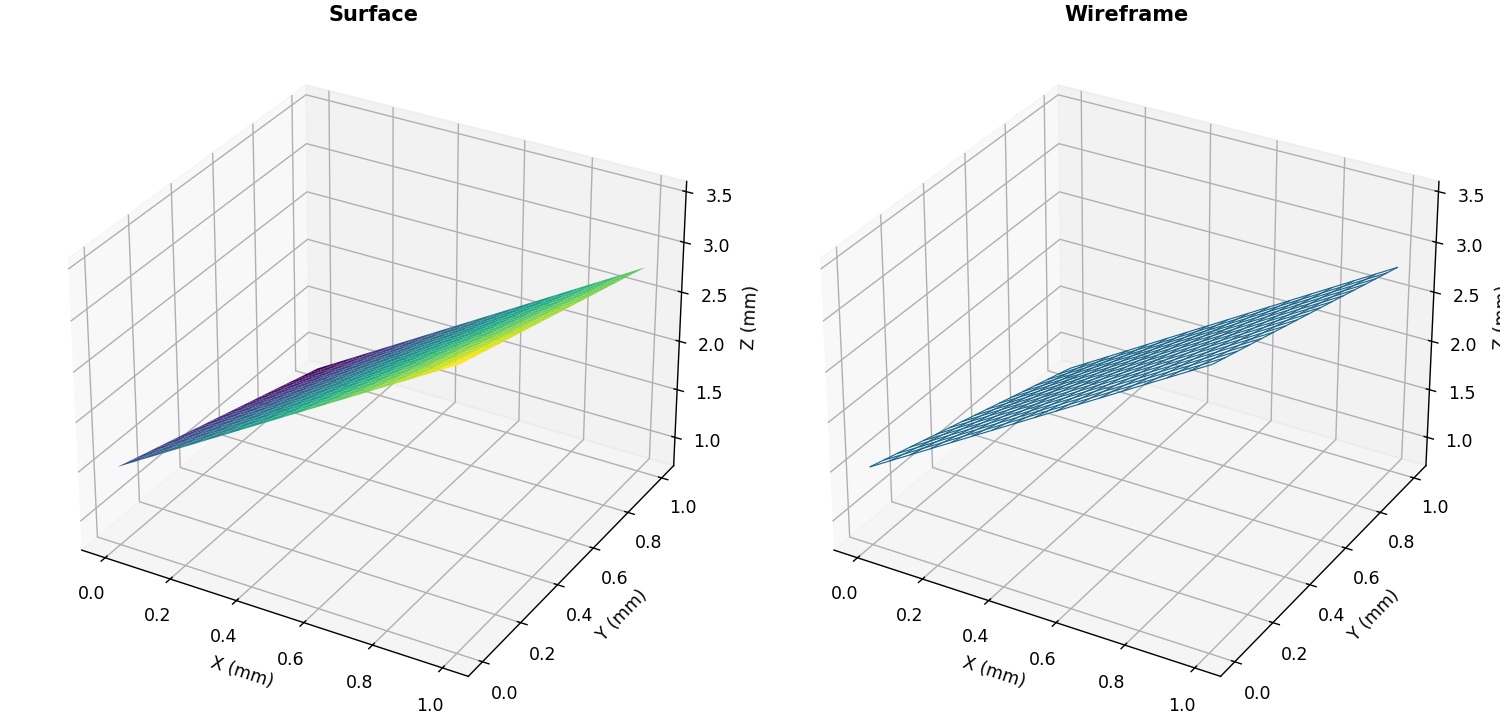
If the integrated 3D view is blocked, plot the same expression outside GX-TXT. Run Export model…, open the output folder and use the following NumPy and Matplotlib example. Match the bounds to the retained domain and the labels to the X, Y and Z units. For the calibration plane, both input axes run from 0 to 1 mm.
import numpy as np
import matplotlib.pyplot as plt
from fit_surface import fit_surface

x = np.linspace(0, 1, 17)
y = np.linspace(0, 1, 17)
xx, yy = np.meshgrid(x, y)
predicted = fit_surface(np.column_stack((xx.ravel(), yy.ravel())))
zz = predicted[:, 2].reshape(xx.shape)

fig = plt.figure()
ax = fig.add_subplot(projection="3d")
ax.plot_surface(xx, yy, zz, cmap="viridis")
ax.set(xlabel="X (mm)", ylabel="Y (mm)", zlabel="Z (mm)")
plt.show()
For a wireframe, replace ax.plot_surface(...) with ax.plot_wireframe(xx, yy, zz). Both views use the exported model values evaluated at your grid nodes.