Self-Built Injection Transformer: First Loop Gain Measurements and Calibration Test Bench

When I design or build a regulated power supply, one of the checks I am most interested in concerns the stability of the feedback loop. It is not enough for the circuit to regulate the DC voltage correctly: it is also important to know how it reacts to variations occurring at different frequencies.

In particular, I want to know up to what frequency the loop gain remains high and where it falls to 0 dB. At lower frequencies the feedback must be effective enough to quickly correct load variations and disturbances; as the frequency increases, however, the gain must progressively decrease, preventing the circuit from trying to correct components that are too fast and risking turning negative feedback into a source of oscillation.

To perform this check, the loop must be slightly perturbed with a variable-frequency sinusoidal signal and the way this perturbation propagates on the two sides of the injection point must be measured. This requirement led to the board described in this article.

The gain value alone, however, is not sufficient: near the crossover frequency it is equally important to observe the phase, on which the stability margin of the system depends.

In a regulated power supply, feedback continuously compares the output voltage with a reference value. If, for example, the output voltage tends to increase, the control circuit reacts in a way that reduces it; if it tends to decrease, it reacts in the opposite direction. This behavior is what makes the feedback “negative”: the correction always tends to oppose the variation that generated it.

This correction, however, is not instantaneous. Transistors, operational amplifiers, compensation capacitors, and other circuit elements introduce delays that, when observed in the frequency domain, appear as an increasing phase shift.

Let us then imagine slightly perturbing the output with a sine wave. At low frequency the circuit is able to follow it and generates a correction in the proper direction, opposing the perturbation. As the frequency increases, the correction arrives progressively later. If the overall delay reaches about 180°, the correction can become practically inverted relative to what is desired: instead of opposing the perturbation, it tends to reinforce it.

This alone is still not sufficient to cause oscillation. The loop gain must also still be high enough at that frequency. If, after one complete trip around the loop, the signal returns with an amplitude equal to or greater than the initial one and with a phase that reinforces it, a small perturbation can persist or grow instead of dying out.

For this reason, when studying the stability of a power supply it is not enough to know only how much gain the loop has, but to observe magnitude and phase. In particular, it is important to identify the frequency at which the gain falls to 0 dB, that is, becomes unity, and to verify how far the phase still is from the critical 180° condition. This distance is the phase margin.

A very slow loop may be easy to make stable, but it will correct fast variations poorly; a loop that is too fast may instead maintain high gain up to frequencies at which the phase delay has already become significant. Compensation therefore serves to obtain a circuit that is sufficiently fast while maintaining an adequate stability margin.

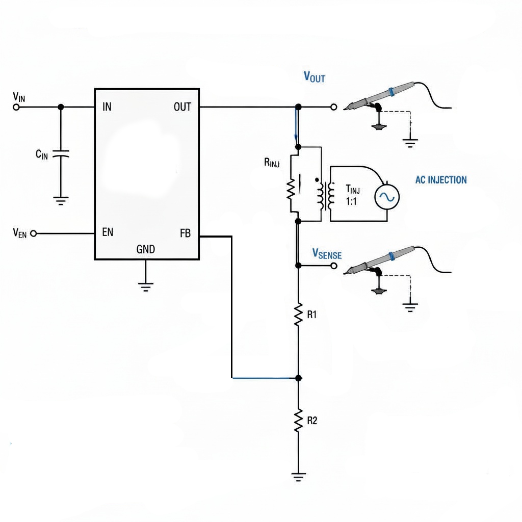
It can be used both with a discrete-component linear regulator and with integrated regulators that provide access to the feedback network, such as an LM2596-ADJ, and more generally with many circuits in which the feedback loop can be appropriately identified and interrupted.

Example of inserting the injection transformer into the feedback loop of a regulator with an external feedback divider. The AC signal is applied between VOUT and VSENSE, while the DC path through RINJ remains unchanged.

Board description

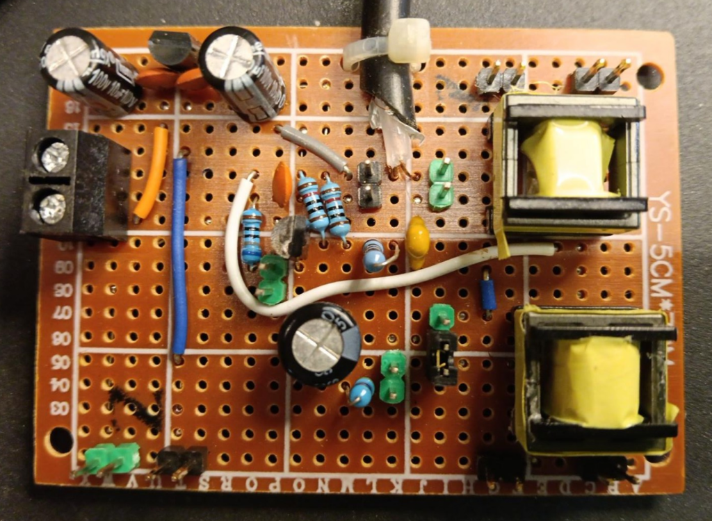
The prototype was built on perfboard and includes the power-supply circuit, the buffer stage that drives the transformer, and the two injection transformers.

The board is powered at 15 V from the bench power supply. The voltage is then locally regulated to 12 V using a 78L12, providing the driver stage with a stable supply. A socket is also available in the lower-left area of the board from which the regulated 12 V can be taken directly, useful for powering auxiliary circuits during testing.

The driver stage uses a 2N3904 configured as a common-collector buffer, or emitter follower. Its purpose is not to provide voltage gain, but to drive the transformer primary with a lower impedance than that of the generator.

The transistor base is biased by two 10 kΩ resistors, which set the operating point at approximately half the supply voltage, therefore around 6 V. Consequently, allowing for the base-emitter voltage drop, the emitter sits at approximately 5.3 V. The emitter resistor is 560 Ω.

The signal from the function generator enters the board through a shielded cable connected near the transistor base. The center conductor carries the signal, while the shield is connected to board ground. The signal is coupled to the base through a 1 µF ceramic capacitor and a 100 Ω series resistor, used to limit base current and provide slight isolation between the generator and the stage.

The signal at the emitter is sent to the transformer primary through a 100 µF electrolytic capacitor, which prevents the DC component from reaching the winding. A 4.7 Ω resistor is also connected in series with the primary to provide slight damping and reduce possible ringing or high-frequency interference.

As far as possible in a perfboard implementation, the ground connections were arranged in a star-ground configuration, avoiding unnecessary sharing of the same return paths among different signals. The shield of the cable from the generator is therefore also returned to the board’s common ground point.

Finally, the two injection transformers are mounted in the lower part of the board. Both are built on EE13 cores and are intended to be compared during characterization of the system.

The injection transformer

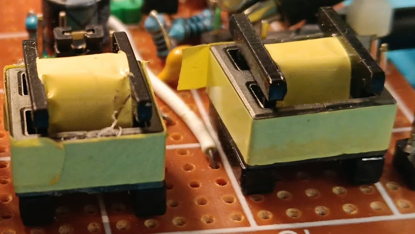
For the transformer I used an EE13 ferrite core, PC40 material, 2+4 configuration, with its corresponding bobbin. The windings were wound by hand using 0.1 mm enamelled copper wire.

I built two transformers with a 1:1 turns ratio but with different characteristics.

The first uses 50 turns on the primary and 50 turns on the secondary. The second instead uses 200 turns on the primary and 200 turns on the secondary, obtained by making, for each winding, four layers of 50 turns.

On the primary side, one end of the winding is connected to a selection jumper, which allows either transformer to be selected. The other end is returned directly to the central ground point of the board. In this area as well I therefore tried to keep the current return separate from the other connections, routing it to the common ground according to the star-ground arrangement used in the prototype.

Building the transformer with 200 turns per winding inevitably introduces some geometrical asymmetry. Because it consists of several stacked layers, the beginning and end of the winding do not occupy equivalent positions relative to the primary, the core, and the other conductors. As a result, the distributed parasitic capacitances are not perfectly symmetrical either.

This effect becomes particularly interesting at higher frequencies: when the two secondary terminals are reversed, the measured response is not perfectly identical. This is one of the aspects I subsequently investigated using the calibration test bench.

Preliminary transformer characterization

Before using the transformers for feedback-loop measurements, I quickly checked their bandwidth. For this test I connected the primary directly to the function generator, set to 1 Vpp, and the secondary to the oscilloscope.

By varying the frequency I observed the ratio between the signal applied to the primary and the signal present on the secondary, identifying on one side the low-frequency region where significant attenuation began to appear and, on the other, the high-frequency region where the transformer’s own resonances became evident.

The 50+50-turn transformer proved usable approximately between 50 kHz and 10 MHz.

The 200+200-turn transformer instead has a substantially flat response starting at approximately 500–700 Hz and remains readily usable to at least 1 MHz. Although it continues to transfer the signal beyond this frequency, for measurements I do not plan to use it above approximately 2 MHz, where parasitic effects and resonances start to become more important.

This test was intended solely to quickly establish the approximate operating bandwidth of the two transformers; their influence on magnitude and phase measurements is instead evaluated later using the calibration test bench.

Calibration test bench and injection-signal amplitude

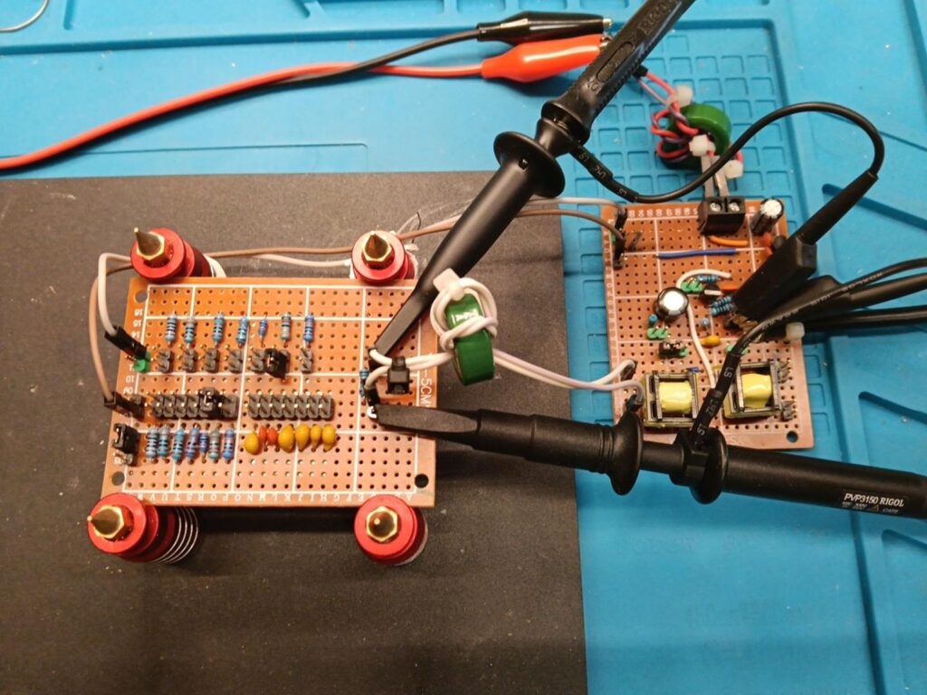
To characterize the board, I built a calibration test bench using several resistive and capacitive networks, then compared the experimental results with the corresponding LTspice simulations.

During testing I also checked the maximum signal amplitude to apply to the transformer primary. As the generator amplitude is increased, the signal injected into the DUT can begin to distort, especially under conditions where the impedance seen by the transformer is lower. This effect becomes particularly evident at lower frequencies, where some of the tested networks present a lower impedance.

To keep the measurement procedure uniform, I therefore chose to use 300 mVpp at the output of the function generator. This is the maximum value that, in the configurations considered, produced a signal on the DUT that was still clearly measurable and free from appreciable distortion.

Reducing noise in the measurement setup

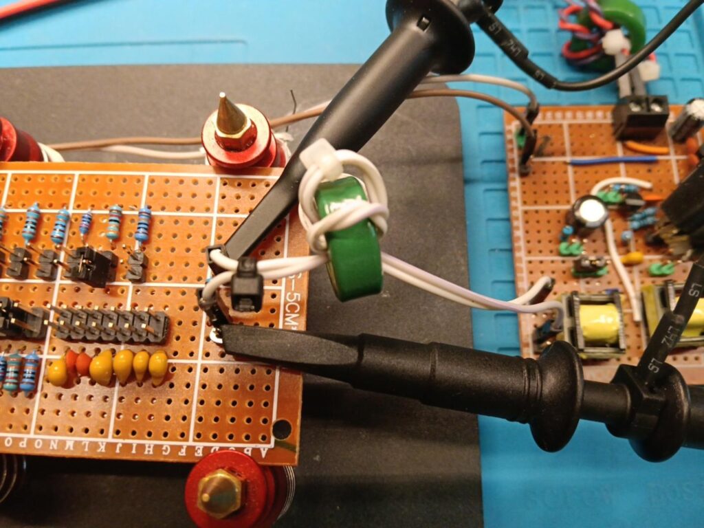
Under some conditions, the signals on the two sides of the injection point can fall to approximately 20–30 mVpp. At these levels, noise picked up by the wiring and common-mode components can become comparable to the useful signal and affect the phase measurement in particular.

For this reason, I tried to minimize interference and, in particular, to carefully control the ground paths. The grounds of the oscilloscope channels are internally common, so I avoided connecting the ground clips of the two probes separately at different points in the circuit and used a single ground reference, connected to the shield braid of the signal cable. This avoids introducing additional return paths and reduces the possibility of creating ground loops that could pick up interference or alter measurements performed on signals of only a few tens of millivolts.

I also kept the power cables as far away as possible from the signal paths. On the more sensitive connections I added some high-permeability Mn-Zn ferrite toroidal cores, passing the cable through the core several times.

The purpose of these toroids is to increase the impedance to high-frequency common-mode components and therefore reduce interference picked up by the wiring, without directly affecting the differential signal being measured.

The calibration test bench

To verify the behavior of the injection board under controlled conditions, I built a small perfboard calibration test bench, consisting of a set of resistors and capacitors selectable by jumpers.

The purpose of the test bench is to create very simple and easily modeled circuits, so that the measurements obtained on the bench can be directly compared with the response predicted in LTspice. To make the comparison as realistic as possible, in the simulation I use the actual component values measured with the LCR meter rather than relying only on nominal values.

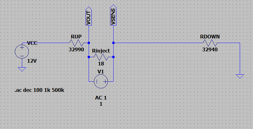
The structure of the test bench is deliberately simple. In the resistive configuration, two resistors are selected, one in the upper branch and one in the lower branch, while the injection point is located in the central area of the network, between the two nodes on which the measurements are made.

This allows me to easily change both the ratio between the two resistors and the overall impedance seen by the transformer, verifying how much the board response depends on the load conditions.

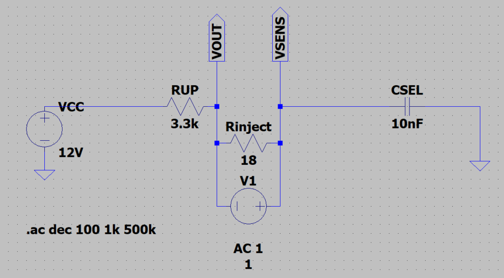
The test bench also includes a set of selectable capacitors, which make it possible to replace the lower resistive branch with a capacitive load. This second configuration is particularly useful because it introduces a strongly frequency-dependent impedance and therefore makes it possible to observe the behavior of the measurement chain under conditions closer to those that may occur in an actual feedback circuit.

For each configuration, the corresponding circuit is built in LTspice and the plot obtained from simulation is compared with the one derived experimentally. The two simplified schematics shown in the following figures illustrate the injection-point connection in the resistive and capacitive configurations.

Components used in the calibration test bench

The test bench provides seven values for the upper resistive branch (RUP), seven for the lower branch (RDOWN) and seven selectable capacitance values. Before starting the measurements, I individually characterized the components with the LCR meter and, in the LTspice simulations used for comparison, entered the actual measured values, rather than the nominal ones.

Position	Measured RUP	Measured RDOWN	Measured capacitance
1	99.94 Ω	99.8 Ω	99.17 pF
2	323.8 Ω	324.4 Ω	463.5 pF
3	995.7 Ω	999 Ω	2.17 nF
4	3.26 kΩ	3.29 kΩ	10.22 nF
5	9.980 kΩ	12.01 kΩ	4.36 nF
6	32.990 kΩ	32.94 kΩ	94.88 nF
7	99.77 kΩ	99.33 kΩ	860 nF

For this first implementation I did not select components specifically intended for precision measurements. In particular, the capacitors were not chosen as C0G/NP0 devices and the resistors were not selected for a low temperature coefficient.

The choice is intentional: the test bench was built on perfboard as an exploratory instrument, with the initial purpose of understanding the behavior of the injection board and obtaining an initial practical characterization of the power supplies and regulators I build. At this stage I am mainly interested in verifying the magnitude and phase trends, identifying the main sources of error, and establishing the actual limits of the measurement system.

For this reason, instead of immediately seeking precision components, I preferred to measure the components actually installed and use the same values in the LTspice simulations. This still allows a consistent comparison between the real circuit and the model.

A later version of the test bench could eventually be built on a PCB, using low-temperature-coefficient resistors, more stable capacitors, and a more controlled connection layout. Characterization of this first prototype will also help determine which of these improvements are actually necessary.

Processing measurements with GNU Octave

For data processing I chose to use GNU Octave, so that I would not have to manually derive amplitude and phase from oscilloscope screenshots and, above all, so that I could apply the same procedure to all measured frequencies.

For each frequency set on the generator, I save the traces of the two oscilloscope channels in CSV format. In my case I use a Rigol oscilloscope: in addition to the samples from the two channels, the file contains the information needed to correctly reconstruct the time axis, such as the initial time and the interval between two consecutive samples. The script uses these data to reconstruct the acquisition time sequence.

The measurement is not derived from peak values or zero crossings. Since I already know the exact frequency set on the generator, a sinusoidal fit at the known frequency is performed on the acquired samples. In this way the amplitude and phase of the two signals are determined separately and, from the complex ratio between the two fundamental components, the magnitude in dB and the phase difference are obtained directly.

The current version of the script also allows a selectable number of harmonics to be included in the fit. I can therefore choose, for example, to use the fundamental, second, and third harmonics, or increase or reduce the number depending on the acquisition. The higher harmonics are used only to describe the waveform more accurately and to prevent distorted components from influencing the estimate of the fundamental; the Bode plot continues to be calculated using only the fundamental component.

It is also possible to choose whether to process the entire CSV file or only a specified number of cycles. This can be useful when the acquisitions are particularly long: the files generated by the oscilloscope can in fact become quite large.

The two A and B measurement series

For each test-bench configuration I initially run the entire frequency series while maintaining a given polarity of the transformer secondary. After completing this first series, I physically swap the two secondary connections and repeat the same measurements.

This produces two series, which I simply call A and B.

The batch macro uses a table in which, for each frequency, the filename for measurement A and, when available, the filename for measurement B are specified. The second acquisition is not mandatory: if it exists it is processed together with the first, otherwise only measurement A is used.

In the current version of the script, when both acquisitions are available, an A/B average is also calculated. This part of the processing is still under investigation: reversing the secondary has shown interesting and repeatable effects, but the dependence on frequency and on the impedance connected to the transformer still needs to be characterized more completely. For this reason, at present I consider this processing an investigative tool, not yet a definitive measurement correction. The results will be discussed in a subsequent article.

Comparison with LTspice

For each test-bench configuration I also build the corresponding circuit in LTspice, using the actual measured component values. I then export the Bode-plot data from the simulator.

The Octave macro imports both the experimental results and the LTspice results. Since the frequencies generated by the simulation do not necessarily coincide with those selected for the measurements, the simulated values are interpolated, on the logarithmic frequency scale, at the points corresponding to the actual acquisitions.

For each frequency, the following can therefore be compared directly:

• measured magnitude and LTspice magnitude;
• measured phase and LTspice phase;
• difference in dB;
• difference in degrees.

The script also calculates the mean error in magnitude and phase.

At the end of processing, magnitude and phase plots and a text file are generated automatically, containing the results of the individual acquisitions, the A and B series, the resulting curve, and the main summary data. In this way, a series consisting of many dozens of acquisitions can be processed uniformly without having to manually transcribe values from the oscilloscope.

Download the scripts

At the end of the article I will make available the GNU Octave scripts used for these tests, together with the instructions needed to prepare the input files and run the processing.

The data-import routine was written specifically for the CSV format exported by the Rigol oscilloscopes that I use. Oscilloscopes from other manufacturers may save traces using different headers or structures, so I cannot guarantee direct compatibility.

If someone wants to use the scripts with a different instrument, they can contact me and send the header and a short excerpt from a CSV file produced by their oscilloscope; where possible I can adapt the part of the script responsible for importing the data.

I do not, however, include the complete acquisitions used during my tests. With the memory settings I use, a single CSV can occupy approximately 16 MB and a single characterization can easily require around forty files: publishing hundreds of megabytes of raw traces would therefore have little practical value. The instructions and scripts are sufficient to repeat the processing using your own acquisitions.

From the first tests to the calibration test bench

Before building the calibration test bench, I carried out a series of preliminary tests using a small board based on an LM358. At present I use only one of the two operational amplifiers available in the IC, but the board was also built as a small test circuit to be reused later for further frequency-response experiments.

The installed IC is a LM358 Texas Instruments and in the LTspice simulations I used the model from the same manufacturer. The external network makes it easy to modify the circuit response; in the first tests I used C5 values of 1 nF, 4.5 nF, 10 nF, and 22 nF, comparing the measured plot each time with the one obtained from simulation.

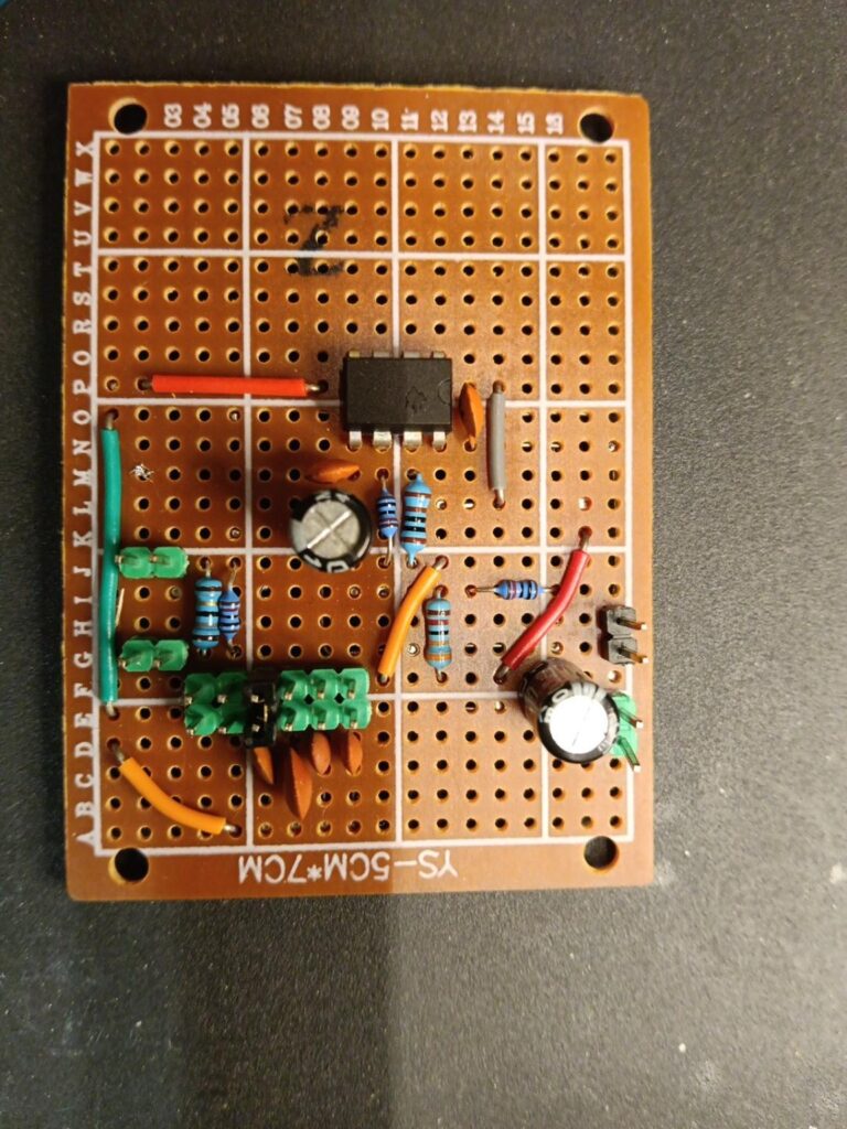
These measurements were essentially exploratory. At this stage I also varied the generator amplitude from one test to another, trying to obtain a signal on the DUT that was large and clean enough to be measured reliably.

These initial tests were already very useful. The 50+50-turn transformer almost immediately proved less suitable, under the conditions and over the bandwidth of interest to me, than the 200+200-turn transformer; I therefore focused the subsequent tests on the latter.

A particularly encouraging result was obtained with C5 = 10 nF. Although this was still a preliminary measurement, the experimental magnitude and phase trends followed the LTspice prediction fairly well. The mean absolute magnitude error for this series was approximately 1.39 dB

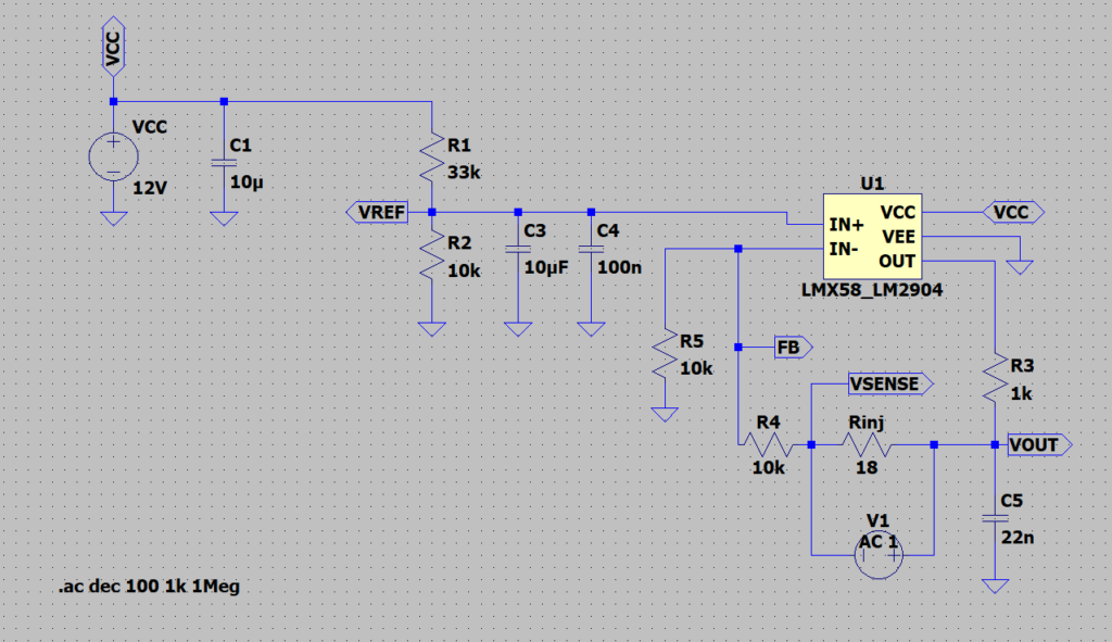
Preliminary comparison between the LTspice simulation and the measurement on the LM358 test board with C5 = 10 nF, using the 200+200-turn transformer. The curves already show encouraging agreement and confirmed the overall validity of the method, while also highlighting the need for a subsequent, more rigorous calibration.

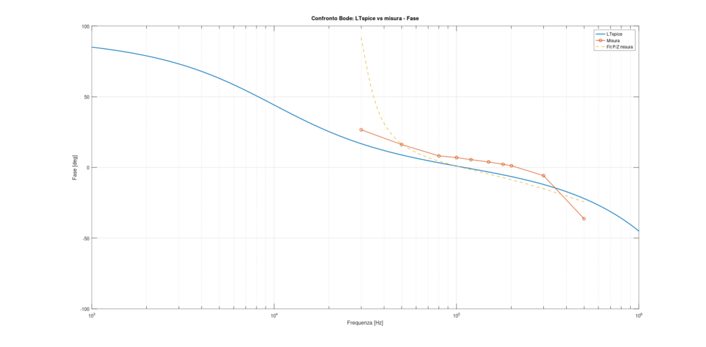
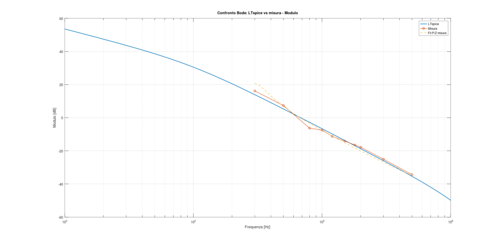
These results were sufficient for me to conclude that, at least qualitatively, the injection system was actually measuring what I was interested in. At the same time, a small systematic deviation was already visible, particularly in phase, which at that point I was not yet able to attribute with certainty to a specific cause.

The test with C5 = 22 nF was instead the first warning sign. The comparison with LTspice deteriorated significantly: in the series performed, the mean magnitude error increased to approximately 6.1 dB, with substantial differences over a large part of the measured bandwidth.

I do not consider these older acquisitions to be a characterization of the system: they were exactly what they were intended to be, namely exploratory tests. They were nevertheless sufficient to make me realize that the response of the injection chain depended on the conditions presented by the DUT and that, before using it confidently on my power supplies, it had to be studied in a more controlled way.

This requirement led to the calibration test bench.

The first measurements on the test bench and secondary reversal

The first tests on the new bench were carried out using an almost symmetrical resistive network, with RUP and RDOWN of approximately 3.3 kΩ.

Because this configuration is extremely simple and easily reproducible in LTspice, it allowed me to notice a phenomenon that had been much less evident in the earlier LM358 tests: the response changed when the two terminals of the transformer secondary were reversed.

The effect was repeatable. It was therefore not simply measurement scatter, but a real asymmetry in the injection system. A hand-wound transformer, especially the 200+200-turn version built using several layers, is not geometrically perfectly symmetrical: reversing the secondary changes the relationships between the windings and the parasitic capacitances.

At this point I changed the measurement procedure.

For each configuration I run the entire frequency series with the secondary connected in one orientation, obtaining what I call series A. After completing the sequence, I physically swap the two secondary leads and repeat the same acquisitions, obtaining series B.

The Octave script handles both series and, when measurement B is also available, the current version calculates the average of the two results.

With the resistor pair of approximately 3.3 kΩ this simple operation produced an extremely interesting result: the deviations for the two polarities were largely opposite, and their combination produced a plot almost exactly overlapping the one predicted by LTspice.

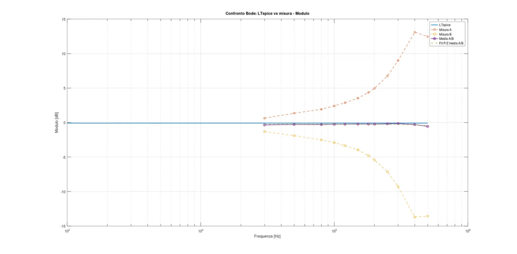
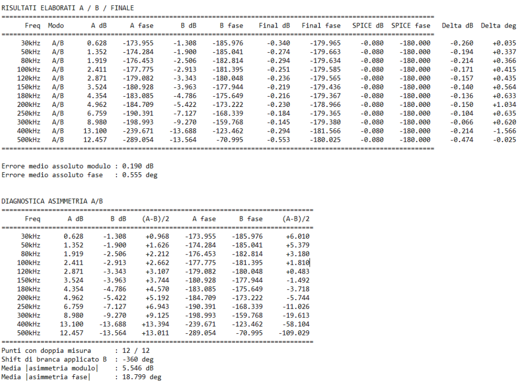
This result could also explain at least part of the small systematic phase error observed during the earlier LM358 tests: in those acquisitions I used only one transformer polarity, so any asymmetric contribution remained fully present in the result.

It would have been very convenient to stop here and conclude that it was always sufficient to make two acquisitions and average them. The next test showed that the situation is more complex.

The 33 kΩ case

Repeating the same procedure with RUP and RDOWN of approximately 33 kΩ, the behavior was significantly worse.

Here too, reversing the secondary reveals an asymmetric component, but the A/B average no longer matches the response predicted by the simulation. A component of the error therefore remains present in both secondary orientations and cannot be eliminated by reversal.

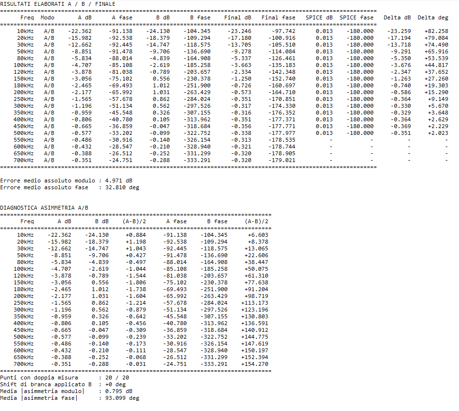
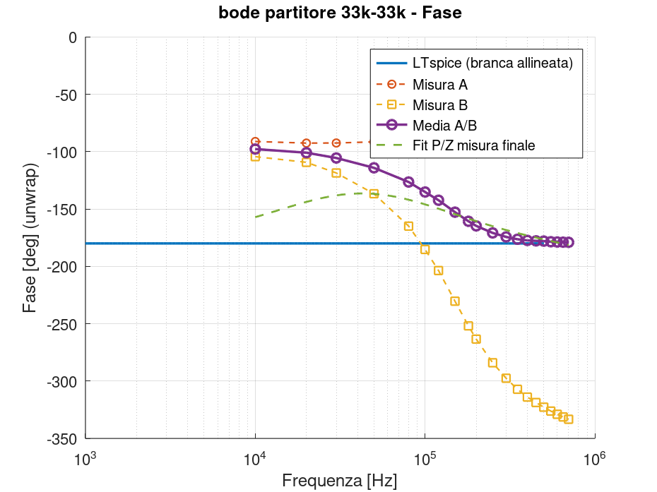
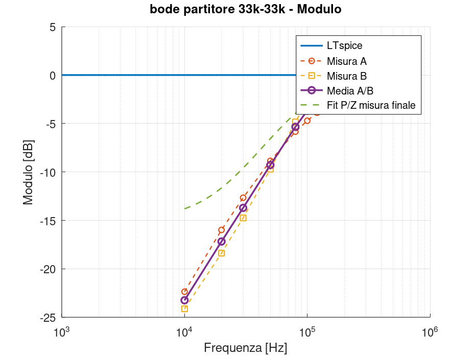
At present, this is one of the most interesting points of the characterization. The tests indicate that there are at least two different contributions: one related to transformer asymmetry, which changes sign when the secondary is reversed and can therefore be strongly reduced by combining A and B, and a second contribution common to both measurements, which becomes important under certain impedance conditions.

I do not yet have enough information to fully describe this latter phenomenon, so I prefer not to turn an experimental observation into a premature conclusion.

This is where I restart with a more controlled measurement

There is also another variable I want to eliminate. In the preliminary tests with the LM358 board I changed the generator amplitude depending on the configuration, in order to obtain signals that were easy to measure.

For the new characterization of the test bench I will instead use a constant 300 mVpp at the generator output for all configurations. This is the lowest value I had already used in the LM358 tests and, in the checks performed so far, it still provides measurable signals while avoiding the distortion that can appear when the injection level is increased excessively.

In this way, frequency and DUT impedance will remain the main variables of the experiment, while the level applied to the primary will remain unchanged.

The current situation is therefore this: the system has already shown that it can produce results very close to the simulation, the dual A/B measurement has highlighted and in some cases almost completely compensated for the transformer asymmetry, but the higher-impedance tests show that the characterization is not yet complete.

And this is precisely where the next measurements will continue.

Download

For anyone who wants to repeat the measurements or use the same processing procedure, I am making available the GNU Octave scripts used during these tests, together with an example file for organizing the acquisitions and the corresponding instructions.

The scripts are the ones I use directly on the bench and are therefore published in their current state of development. In particular, the handling of the dual A/B measurements and some processing steps are still being verified and may be updated as the characterization progresses.

The available files are listed below:

• Octave script for batch processing of the measurements
• Example CSV table for organizing the acquisitions
• Instructions for using the script

The complete CSV files from my acquisitions are not included because they can reach approximately 16 MB each and a single test series can require several dozen of them.