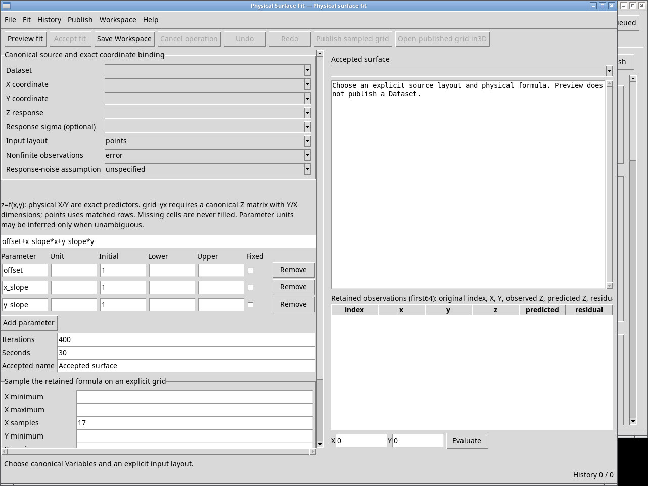
Open Surface Fitter
Open the viewer from the catalog
Open a GX-TXT Session containing the canonical Dataset you want to analyze. To follow the exercises, import the practice Datasets before opening the viewer. On the Viewers tab, click the Surface Fitter tile. The window is titled Physical Surface Fit and shows the Workspace name. This manual uses the labels shown in the interface.
Import the practice Datasets
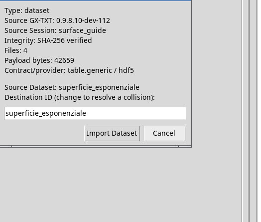
Download the ZIP package you need. In an open Session, switch to the Dataset tab and open Dataset actions on the browser toolbar. Choose Import Dataset ZIP… and select the ZIP file. In the verification dialog, keep the suggested Destination ID to follow the examples exactly. If the ID is already in use, choose an unused one and substitute it throughout the exercise. Click Import Dataset and check that the confirmation says Integrity: verified.. Cancel closes the dialog without importing. Open Surface Fitter after importing, or reopen it if the new ID is missing.
- Calibration plane for the first fit, known-sigma estimation and XY evaluation.
- Y/X grid to verify the 4 × 5 shape.
- X/Y grid to reproduce rejection of the reversed dimensions.
- Y/X grid with a missing cell to compare error and omit.
- Points with a missing measurement to see which source indices are retained.
- Quadratic surface for an expression with six parameters.
- Exponential surface for a fixed offset and bounded length scales.
Find your way around the window
- Action bar
- Preview fit computes a preview, Accept fit keeps the fit, Save Workspace saves the current settings, and Cancel operation cancels a running fit. Use Undo and Redo to navigate History. Publish sampled grid and Open published grid in3D require an accepted fit.
- Settings and results
- Drag the divider to give the pane you are reading more space. Scroll down on the left to Sample the retained formula on an explicit grid to set the output grid. On the right, scroll the report and residual table.
- Status and History
- Read the status line after each command. At startup, History 0 / 0 indicates an empty history. A disabled command may require a fit result, a valid position in History or a running calculation.
First exercise: fit a calibration plane
- Select
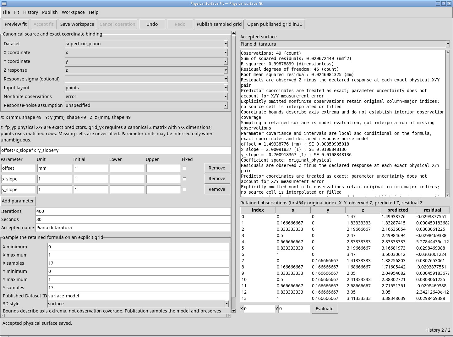
superficie_pianoas Dataset. Bindx,yandzin their respective selectors. The Dataset contains 49 synthetic measurements in mm. Choose points, error and unspecified. Leave Response sigma (optional) blank for this first fit. - Keep the initial expression
offset+x_slope*x+y_slope*y. You can specifymm,1and1as the parameter units, respectively. Keep Initial at 1 and leave the bounds blank. - Click Preview fit. Check for 49 observations and an RMS error close to
0.0246 mm. Expect about 1.4994 mm foroffset, and slopes of about 2.0009 and −0.7009. - Enter a name in Accepted name, for example Calibration plane, and click Accept fit. Select that name on the right, enter
0.4and0.6in X and Y, and click Evaluate. The status line should show a result close to1.8792 mm.