

Publish, Visualize and Export
Publish the canonical field
In Results → New field Dataset ID, enter an unused ID such as guida_campo_elettrico. The field starts with em_field. Use Reset to restore that value.
With a completed job for the current scientific model, press Publish field in the tab or choose Results. The Studio publishes the cell Dataset with the chosen ID and the node Dataset with suffix _nodes. In Solve, look for Published exact canonical node/cell fields. The command selects the cell Dataset. If Publication requires two unused canonical Dataset identities appears, make sure both IDs are available and try again.
Select and browse a Dataset
Open Canonical tabular Dataset in the Results tab. The list shows compatible canonical tables. Use Inspect Dataset table, also available in the Results menu, and select the Dataset table tab on the right. Check the ID, format and row range in the top line. This read-only view also works for tables from outside the FEM workflow. Scientific field views use the cell Dataset with its connected node Dataset.
- Previous page
- Go to the previous page. This action is disabled on the first page.
- Next page
- Go to the next page. The example uses 100 rows per page. This action is disabled on the last page.
- Go to source row / Go
- Enter a source row number starting at 1 and press Go. In this example,
350opens rows 350–449. - Column details
- Opens the declared schema below the grid. Scroll to see names, units and metadata. Hide column details returns to the table alone. An item without metadata is marked as undeclared.
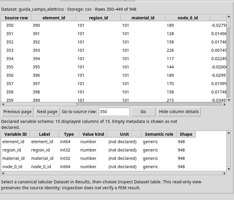
node_0_id, node_1_id and node_2_id columns refer to the original nodes.Celle. element_id identifies the triangle. region_id and material_id identify the region and material. x, y and z are centroid coordinates in meters. field_x, field_y and field_z are the field components in the field’s units. field_norm is its magnitude. potential is the mean of the cell’s nodal potentials. area is the area in m². Nodi. The other Dataset contains the original node IDs, coordinates and nodal potential.
View the exact field on the cells
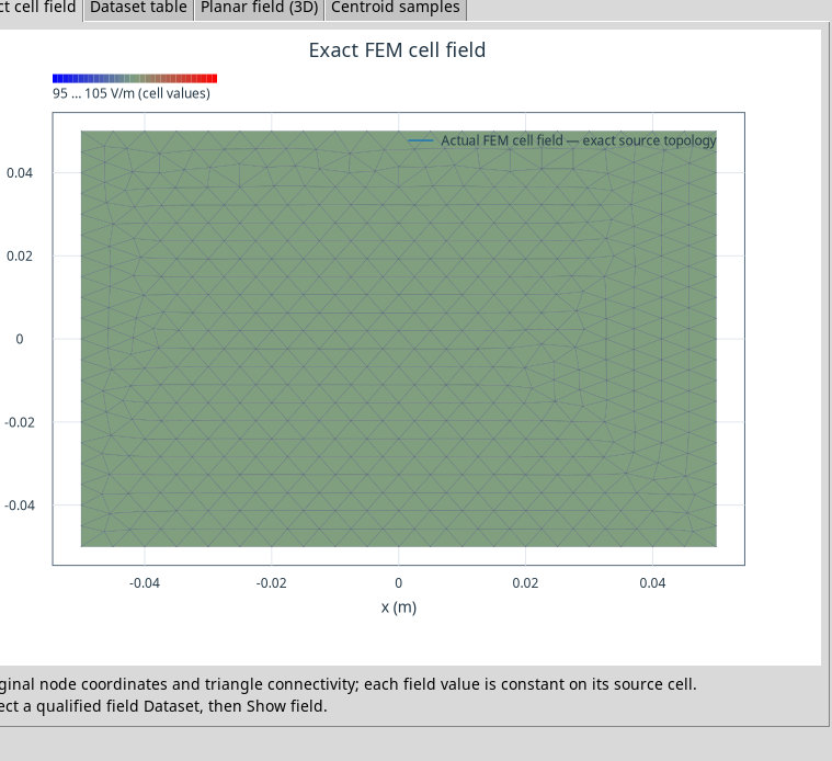
After selecting the cell Dataset, press Show field on the toolbar or choose Results, then switch to Exact cell field. The plot uses the original coordinates and connectivity. For the first-order FEM vector field, the color represents the magnitude, which is constant within each original cell.
Check the source units and the displayed range. If the field is almost uniform, the color range can widen to make the plot readable. For the electrostatic example, the physical value remains about 100 V/m even if the display scale extends beyond the data.
Use the wheel to zoom, drag with the middle button to pan and double-click to restore Fit. The plot continues to use the selected Dataset. To read a specific cell’s value, use its triangle ID to locate the source value in the table.
Compare samples at the cell centroids
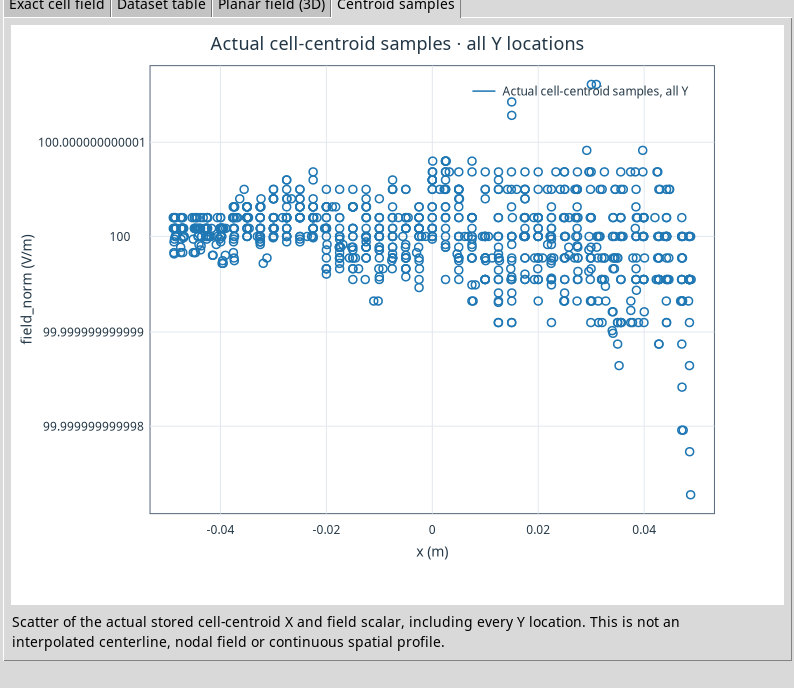
Press Show centroid samples and open Centroid samples. The horizontal axis shows the X coordinate of each original centroid. The vertical axis shows the cell field magnitude in V/m or T. The scatter plot includes cells at all Y coordinates. Each point gives the computed value for its cell. In the electrostatic example, the deviations around 100 V/m are numerical.
View the same cells in Planar field (3D)
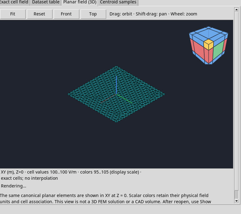
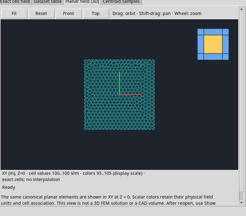
With the cell Dataset selected, use Show planar field in 3D and switch to Planar field (3D). The view uses Z = 0 to display the triangles in XY. Color represents the per-cell field value in its original unit. The geometry remains planar.
- Fit
- Frame the elements of the current scene.
- Reset
- Restore the view’s initial framing.
- Front
- Switch to the front view. Depending on orientation, a scene entirely in the XY plane can appear edge-on.
- Top
- Look along the Z axis to see the entire plane.
- Drag, Shift-drag and Wheel
- Drag to orbit, hold Maiusc while dragging to pan, and scroll to zoom. The controls are grayed out until a scene loads. If Rendering… appears, wait for the update before comparing views.
After reopening, select the canonical Dataset again and press Show planar field in 3D to populate the pane.
Save graphs in Plots
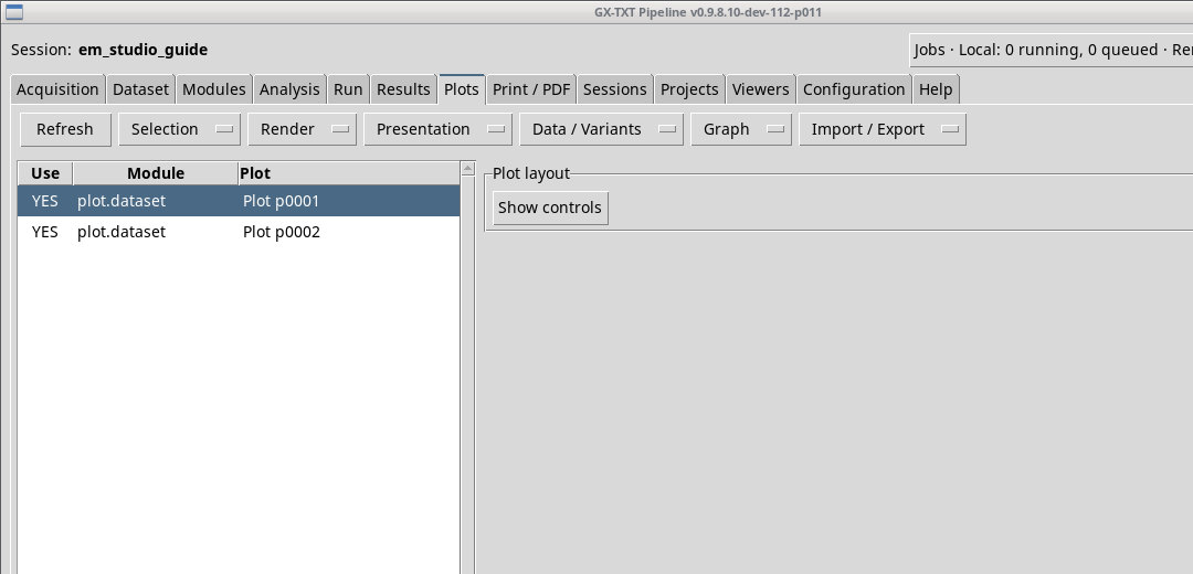
With a canonical field selected, press Publish charts to Plots. The main Plots tab lists two distinct plots, one for the exact field and one for the centroid samples. Both link to the source and can be reopened from the Session’s plots area. Republishing the same source updates those two existing entries.
Export the exact field as a figure
Display the selected field with Show field before choosing Export exact field… from the Results tab or menu. The exact field plot must correspond to the currently selected Dataset. If you change the Dataset, run Show field for that field before exporting.
In the Export native field figure dialog, choose a destination and format. PNG is the default raster format. SVG is an editable vector figure. PDF is a vector document for printing and sharing. If the file already exists, Yes replaces it and No keeps it and takes you back to the destination picker. Cancel closes the dialog without saving an image.