

How an IR Remote Control Works: Carrier, MARK, SPACE and NEC Protocol
GX-TXT-v3 started as a Remote Control Tester: a relatively simple instrument designed to quickly check whether an infrared remote control is actually transmitting.
The initial idea was very simple. I did not want to limit myself to watching the LED flash by directly following the pulses received from the remote control. I only knew that the IR signal was modulated on a carrier around 38 kHz, and I wanted to use those pulses to progressively charge a HOLD network, so that the LED would remain on long enough to be clearly visible.
This also led to the idea of adding a preamplifier stage and threshold adjustment, so that I could obtain not only a simple “transmitting / not transmitting” indication, but also a very basic indication of the received signal strength. I did not want to use either a galvanometer or an LED bar: instead, I wanted to try to derive this information from the LED on-time.
At that point, however, my practical knowledge of an IR remote-control signal essentially stopped there: I knew that a carrier around 38 kHz was present, but I had not yet looked closely at how the command was actually structured on top of that carrier.
It was during the measurements that this began to interest me. By observing the waveforms at different points in the circuit, I realized that behind that simple flashing LED there was a much more interesting timing structure. From there came the desire to go deeper and use the Remote Control Tester not only to check an IR transmitter, but also to understand better what it was actually transmitting.
The Remote Control Tester therefore also begins to become a small experimental front-end for studying IR remote controls. This was not the main function originally planned for the project, but it emerged naturally during the measurements.
In this test I therefore do not want to stop at checking whether the remote control works. I want to use the acquired waveforms to organize and better understand some fundamental IR protocol concepts: carrier, MARK, SPACE, header and bit encoding.
Starting from the received signal
To better understand what an IR remote control is actually transmitting, the most natural starting point is to observe the signal received by the circuit directly.
The first acquisition I consider is the VIR node, that is, the signal coming from the front-end connected to the photodiode. Looking at the entire command over a relatively wide time scale, the waveform initially appears rather complex: groups of oscillations can be seen, separated by intervals in which the signal returns toward its idle level.
Zooming in on the beginning of the command already reveals a structure. There is a first group of pulses that is much longer, followed by a pause that is also relatively long; shorter groups then appear, separated by intervals of different durations.

For the moment I do not assign any meaning to these durations. The important point is to observe that the command is not made up of a continuous sequence of pulses at a constant frequency: the carrier is transmitted in bursts, separated by pauses. It is precisely in the duration and sequence of these intervals that the information transmitted by the remote control begins to appear, and this pattern is what sparked my curiosity: a sequence of groups of signals modulated on a base frequency of about 38 kHz.
To understand it better, I therefore changed the time scale and looked more closely at one of these groups of pulses.
Reading the command directly on the oscilloscope
When I made the first acquisitions, my approach was much more direct: before moving on to any numerical processing, I tried to extract as much information as possible simply by looking at the waveform on the oscilloscope screen.
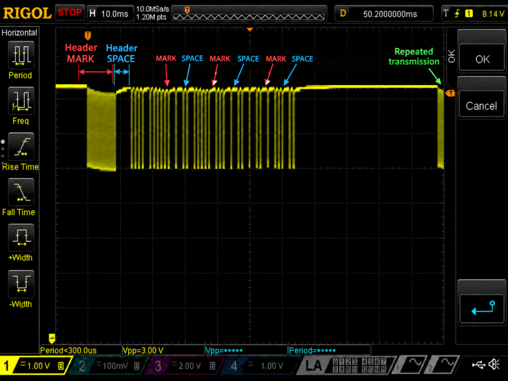
The first thing that struck me was an initial sequence of very closely spaced pulses, dense but still distinguishable. Immediately afterward there was a fairly clear empty interval, followed by a sequence that already looked clearly organized, with groups of pulses separated by pauses of different durations. Even without yet knowing the detailed structure of the protocol, it was difficult not to read that waveform as some form of information encoding.
The initial sequence seemed to have a different function from what followed: an initial section that appeared intended to prepare or synchronize reception, then a pause, and finally the section containing the actual command. Farther to the right, another sequence could also be seen, indicating that the remote control was repeating the transmission.
At that time I had already read about IR protocols and knew that the intervals in which the carrier is present are called MARK, while those in which the carrier is absent are called SPACE. Reading these terms in a theoretical description is one thing; beginning to recognize them in the real waveform displayed on your own oscilloscope is another.
All the subsequent work started from those first observations. I acquired the signals, wrote the scripts needed to identify the carrier, reconstruct the burst sequence, separate MARK and SPACE, measure their durations and finally attempt to identify the protocol.
Today, as I write this article, that signal is no longer new to me: I have observed and analyzed it many times. For that very reason, I think the time has come to stop and take stock properly, returning to the original waveform and putting together in an orderly way what I learned during the work.
What I want to do here is therefore explain calmly how this signal is structured, starting from what can be seen directly on the instrument and progressively moving toward its structure: carrier, MARK, SPACE, timing and finally command encoding.
Two time scales in the same signal
In the same oscillogram I can immediately see two different time scales.
The first is fast: it is the closely spaced succession of carrier pulses.
The second is much slower: it is defined by the duration of the groups of pulses and the pauses that separate them. It is this slower structure that carries the command.
In other words, the carrier is the fast rhythm on which the signal is modulated; the information is contained in the way that carrier is made to appear and disappear over time.
MARK and SPACE
The intervals in which the carrier is present are called MARK.
The intervals in which the carrier is absent are called SPACE.
Looking at the signal this way makes the waveform much easier to read: I no longer need to follow every single carrier pulse, but can instead focus on the duration of the MARK and SPACE intervals.
It is precisely in the sequence of these intervals, and especially in their durations, that the command information is built.
From MARK and SPACE to bits
Once MARK and SPACE have been separated, the next step is to understand where the information is located.
In the signal I am analyzing, the MARK intervals that make up the data have an almost constant duration. What changes clearly is the duration of the SPACE following each MARK.
Here, however, I need to distinguish between what I can understand by looking at the oscillogram and what I can actually measure.
The acquisition time base is 10 ms per division. At this scale the header can be read reasonably well: the initial MARK lasts about 9 ms and occupies almost one division, while the following SPACE lasts about 4.5 ms.
The symbols that make up the data are much smaller. The subsequent measurements show MARK intervals of about 568 µs: on the overall oscillogram this corresponds to only 0.057 divisions. The short SPACE, about 590 µs, is practically on the same scale. The long SPACE, about 1.70 ms, reaches only about 0.17 divisions.
So, by looking at the image, I can immediately infer that pauses of different durations exist; to assign them precise values, however, I need to zoom in on the signal or work on the acquired data.
And it is precisely from these measurements that the encoding structure emerges: the data MARK intervals have an almost constant duration, while the SPACE intervals cluster mainly around two values, one short and one long. In the signal I am analyzing they are about 590 µs and 1.70 ms.
It is this timing difference that encodes the bits: a short SPACE represents one value, while a long SPACE represents the other. In the encoding I am observing, the short SPACE corresponds to 0 and the long one to 1.
The bit, therefore, is not represented by a high or low voltage as on a normal digital line. It is represented mainly by a duration.
Measurements on the real signal
After deriving the general structure of the command directly from the oscillogram, I move on to measurements performed on the acquired data.
I observed the signal at several points in the circuit. The VIR node is very useful because it closely represents the received signal, but it is also a sensitive, high-impedance node. I therefore did not want to depend exclusively on a direct measurement at that point.
Part of the circuit was also designed to bring the signal toward more robust nodes, where I can observe and acquire it under more favorable conditions. This also lets me see how the waveform changes as it passes through the different stages.
In the following sections I therefore take the plots one at a time. Not as a gallery of results, but to understand what each measurement shows and what information I can extract from it.
The command seen through local maxima and minima
To begin the quantitative analysis, I start from a more compact representation of the signal at the VIR node. In this plot I am not showing the complete waveform sample by sample, but rather the evolution of the local maxima and local minima over time.
The meaning is simple. The Local maximum trace represents, in each small analysis interval, the maximum value reached by the signal. The Local minimum trace represents the minimum value reached in the same interval.
When the carrier is present, the signal oscillates with a certain amplitude and the two curves separate clearly. When the carrier disappears, the signal closes back around its mean level and the distance between maximum and minimum becomes much smaller. In this way the command structure remains readable even on a time scale of several milliseconds.
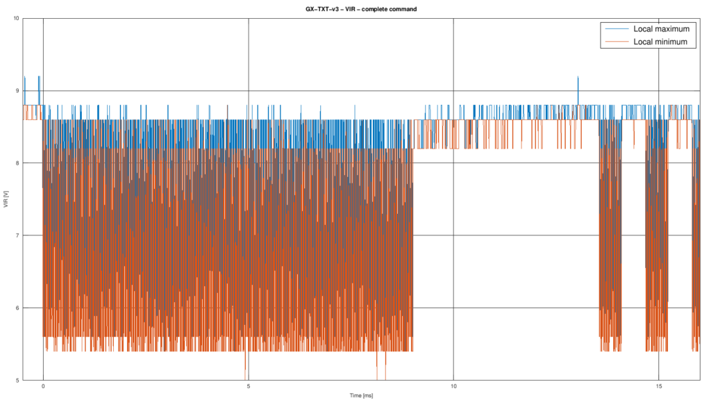
On the right I am not yet observing the entire command, but only the beginning of the data sequence. After the long header MARK and SPACE, the first MARK and SPACE intervals associated with the bits appear: in the displayed section, two complete MARK–SPACE pairs and the beginning of the following MARK can be distinguished.
This zoom is therefore particularly useful because it places on the same plot the two time scales I had recognized on the oscilloscope: on one side the long header, and on the other the first much shorter intervals that begin to build the command data.
Together with the previous oscillogram, this zoom makes the meaning of MARK and SPACE even clearer. In the original signal I recognized them mainly from the overall shape; here they become well-separated timing intervals that are much easier to read.
An important point about the encoding is also clearly visible: in the data section the MARK remains essentially the same duration, while the following SPACE changes. It is therefore mainly the duration of the SPACE that determines the bit value.
In this representation the difference between a short SPACE and a long SPACE is much more evident than in the overall oscillogram. It is precisely this timing difference that allows the two logic values to be distinguished.
Inside a MARK: carrier detail
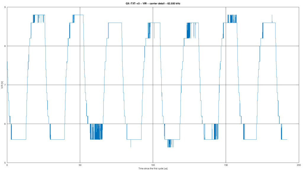
If I zoom in further on the signal at the VIR node, the internal structure of a MARK becomes visible. What appeared on the millisecond scale as a single interval occupied by the carrier is actually made up of a regular succession of oscillations.
The plot shows about 200 µs of signal and therefore only a few cycles. The periodicity is already clear and allows me to move from the scale of MARK and SPACE intervals to the much faster carrier time scale.
The 62.5 kHz value automatically reported in the plot title is incorrect and must be regarded as a processing artifact. A visual check shows this immediately: over an interval of about 200 µs, roughly seven main cycles can be seen, so the frequency is clearly on the order of a few tens of kilohertz, not 62.5 kHz.
Measuring the distance between two consecutive main peaks more carefully gives a period of about 26 µs, corresponding to a frequency of about 38 kHz. The algorithm therefore probably counted some irregularities or small disturbances in the signal as additional transitions, distorting the automatic estimate.
In this case the plot is also useful as a check on the numerical result: the real waveform makes it immediately clear that the value shown in the title is not compatible with the periodicity actually visible.
MARK / SPACE reconstruction of the command
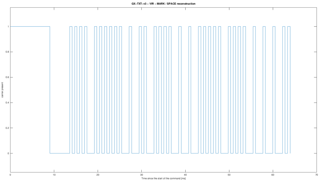
At this point I can remove the individual carrier cycles from the representation and keep only the information I am interested in: carrier present or carrier absent.
In the plot, level 1 therefore indicates a MARK, while level 0 indicates a SPACE. The IR signal thus becomes an extremely simple timing sequence to read.
At the beginning, the long header MARK appears immediately, followed by its corresponding SPACE. After the header, the data section begins: the MARK intervals become much shorter and retain an almost constant duration, while the SPACE intervals separating them can have two clearly different durations.
Here, what I had already inferred from the oscillogram becomes particularly evident: in the data section, it is mainly the duration of the SPACE that encodes the bit. There is no need even to count the intervals one by one to see the structure: the short and long SPACE intervals are immediately distinguishable.
This representation is therefore a kind of bridge between the real analog waveform and the logical structure of the command. The carrier has disappeared from the plot, but exactly the timing information that carries the data remains.
Duration of MARKs and following SPACEs
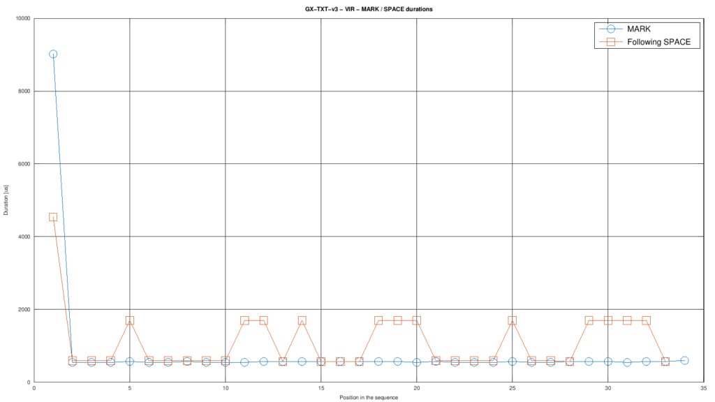
This plot relates, position by position, the duration of each MARK to that of the SPACE that follows it. The horizontal axis gives the order of the intervals in the sequence; the vertical axis gives their duration in microseconds.
The first point immediately stands out from all the others: it is the very long header MARK, followed by the corresponding header SPACE, which is also much longer than the following intervals. This already confirms quantitatively what was visible on the oscillogram only as a more extended initial structure.
After the header, the situation changes sharply. The MARK intervals in the data section all remain concentrated around a similar duration, while the SPACE intervals that follow them clearly divide into two groups. Some have a duration of the same order as the corresponding MARK; others are much longer.
This is where the encoding becomes obvious: the MARK remains almost constant, while the following SPACE carries the information. In other words, the bit is identified not so much by the duration of the carrier burst, but by the pause immediately following it.
I particularly like this plot because it turns into numbers something that had already become clear from the previous images: there are MARK intervals that are almost all the same and two distinct types of SPACE, one short and one long. The command structure therefore emerges very cleanly, without having to follow the details of the analog waveform anymore.
From the IR signal to the circuit measurement points
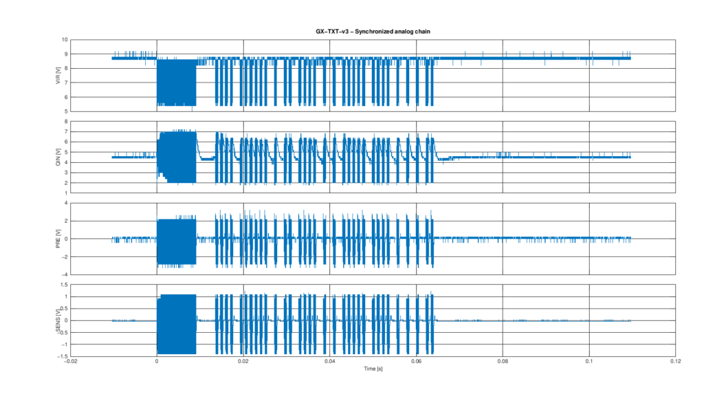
With these two plots I change perspective slightly. So far I have mainly used the VIR node to understand how the IR command is structured. Now I am no longer studying the protocol itself, but the way I can observe and measure that signal through the circuit.
VIR is the most direct and informative point, but it is also a particularly sensitive, high-impedance node. In the GX-TXT-v3 I therefore want to be able to follow the same signal at later points in the chain, where measurement conditions are more favorable. The complete schematic, PCB, Gerber files and other construction details are available in the project articles and files; here I am interested only in seeing what happens to the signal as it passes through the circuit.
The first plot shows VIR, QIN, PRE and SENS simultaneously, using the same time base. The important point is not to compare the absolute voltages directly, because each stage operates with its own bias point, but to observe the timing structure.
The long initial burst and the following MARK/SPACE sequence remain recognizable throughout the chain. The electrical shape changes, as expected when passing through different stages, but the timing structure of the command is preserved. This means I am not forced to extract all the information directly from the delicate VIR node: I can follow it farther along the circuit as well.
The second plot instead compares the excursion from baseline measured at the four points. At VIR I obtain about 3.8 V, at QIN about 2.8 V, at PRE about 3.4 V, and at SENS about 1.44 V.
These values should not simply be interpreted as gains of the individual stages: the nodes have different bias conditions, functions and waveform shapes. The comparison is instead intended to show how much usable signal remains available at the different points in the chain.
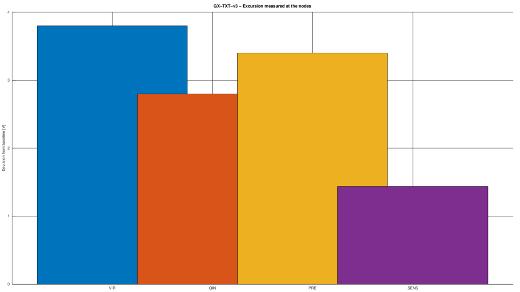
Read together, the two plots therefore show two different but complementary things: the first verifies that the timing information of the command survives through the circuit; the second shows the electrical excursion with which I can recover it at the different measurement points.
Experimental conditions and main values
Before reporting the results, it is important to define the test conditions. The amplitudes observed at the different nodes, and more generally the circuit response, are meaningful only when associated with the configuration used for the acquisition.
| Test manifest | |
|---|---|
| Project | GX-TXT |
| Board / revision | GX-TXT-v3 |
| Test type | catena_veloce |
| Date | 2026-09-02 |
| Remote control | Android TV board |
| Button | OFF |
| Distance | 20 cm |
| P_GAIN | 540 Ω |
| P_SENS | 4980 Ω |
| Supply voltage | 8.962 V |
The acquisition contains 3,000,000 samples, recorded at 25 MSa/s, for a total duration of about 120 ms.
| Quantity | Value |
|---|---|
| Analyzed command duration | about 63.95 ms |
| Detected MARKs | 34 |
| Header MARK | about 9.02 ms |
| Header SPACE | about 4.54 ms |
| Data MARK, median duration | about 568 µs |
| Short SPACE, median duration | about 590 µs |
| Long SPACE, median duration | about 1.70 ms |
| Observed carrier | about 38 kHz |
| VIR excursion | about 3.8 V |
| QIN excursion | about 2.8 V |
| PRE excursion | about 3.4 V |
| SENS excursion | about 1.44 V |
Note: the values reported describe this specific test and must be read together with the corresponding experimental manifest. In particular, the amplitudes at the nodes depend on the distance from the remote control, the settings of P_GAIN and P_SENS, the supply voltage and the transmission conditions.
For the electrical meaning of the VIR, QIN, PRE and SENS nodes, the circuit schematic, PCB, Gerber files and other construction details, I refer to the other GX-TXT project articles and files. For the general structure of IR protocols, I instead refer to the technical sources collected in the project.
Which protocol am I observing?
From the measured timing and the frame structure, the best candidate belongs to the NEC family. The command contains 32 bits and, interpreting the bytes LSB-first, gives 0x08 0x16 0x87 0x78. The final byte is the complement of the command byte, while the address pair does not follow the complementary form of classic NEC. For this reason, the most plausible identification is NEC extended, or in any case a compatible variant of the NEC family.
I do not go into the differences between the various protocol versions here; for that I refer to the technical sources collected in the project. In this page I am mainly interested in showing how, starting from a real oscillogram, it is possible to reach the timing structure and a reasonable identification of the command.
Conclusions
Looking back from the beginning, the path was much simpler than it seemed when I started.
I started from a waveform that, viewed all at once on the screen, said almost nothing: a tangle of oscillations with empty gaps in between. The first step was to realize that there were two different speeds inside it. A fast one, made up of the individual carrier pulses around 38 kHz, and a slow one, made up of the groups of pulses and the pauses separating them. From that point on I could stop looking at the carrier: it carries the signal, but it does not tell the story.
Staying on the slow time scale, everything reduced to just two conditions: the carrier is present, or the carrier is absent. MARK and SPACE. The signal became a sequence of filled and empty intervals, and at that point the only thing left to look at was how long they lasted.
And this is where the command emerged almost by itself. The first interval is long, about 9 ms, followed by a pause of about 4.5 ms: this is the header, the signal that tells the receiver that something is about to arrive. After the header, all the MARK intervals become equal, about 568 µs each, and stop carrying information: they simply act as a beat. What changes is the pause following each one, which can be about 590 µs or about 1.70 ms. Short pause, zero. Long pause, one.
Counting the intervals makes everything line up cleanly: 34 MARK intervals in total, namely the header MARK, the 32 data MARKs, and one final closing MARK whose only purpose is to delimit the pause of the last bit. Thirty-two bits, therefore four bytes, which in this command are 0x08, 0x16, 0x87 and 0x78. The last two are complements of each other, and this is worth noting: it is how the receiver checks that it has read the command correctly, because if the two bytes do not correspond, the command is simply discarded.
What struck me most, once I reached the end, is that there is no difficult step. I did not have to decipher anything: I simply kept looking at the same waveform while changing the question each time. First how fast it is, then when it is present and when it is absent, then how long it lasts. Every time I removed one level of detail, a little more structure appeared.
And that is why, if you have reached this point, the result I care about is not that you have learned what my remote control was transmitting. It is that the next time you see an oscillogram of this kind, whether yours or someone else’s, you can begin to read it with the same questions: where is the carrier, where are the MARK and SPACE intervals, which durations repeat. From there, the protocol practically tells its own story.
That was exactly the goal: to take a Remote Control Tester originally built to make an LED flash and use it as an excuse to really look inside the signal of an infrared remote control.