The Koren triode model: theory, parameters and limitations

This article is not about how to obtain a SPICE model from a datasheet: that is the job of the fitting workflow. The goal here is more theoretical: to understand what the Koren triode model actually represents, why its equation has this form, what its parameters mean, and above all where the model stops being trustworthy.

I use the 6BX7-GT fit as a concrete case study. The dataset contains 440 digitized points from the plate-characteristic family, spread across 11 grid-to-cathode voltages from 0 to -50 V. The triode.koren_v1 model was globally optimized in GX-TXT and then translated into an LTspice netlist to verify that the same equation produces the same curve family inside a circuit simulator.

The key distinction to keep in mind throughout the article is:

real tube ≠ Koren model ≠ one particular fitted parameter set. The first is a physical device; the second is a phenomenological family of equations; the third is one approximation built from one particular dataset.

1. From a simple physical law to a SPICE-usable model

A classical starting point for describing the behaviour of a triode is a power law of the form \[ I_a \propto \left(V_{gk}+\frac{V_{ak}}{\mu}\right)^{3/2} \]

valid when the quantity in parentheses is positive; when it becomes negative, the idealized model assumes zero plate current. The \(3/2\) exponent is related to the Child-Langmuir law for space-charge-limited current. In a triode, however, the plate current is controlled not only by the plate voltage: the control grid also has a strong influence on the electron flow.

The quantity \[ V_{\mathrm{eff}} = V_{gk}+\frac{V_{ak}}{\mu} \]

can therefore be interpreted, in this simplified model, as an effective control voltage that determines the plate current. The grid-to-cathode voltage \(V_{gk}\) appears directly, while the plate-to-cathode voltage \(V_{ak}\) is divided by the amplification factor \(\mu\). This makes the stronger control action of the grid immediately apparent.

For example, if a triode has \(\mu=10\), a change of \(1\,\mathrm{V}\) in grid voltage produces, to a first approximation, the same change in \(V_{\mathrm{eff}}\) as a change of \(10\,\mathrm{V}\) in plate voltage. If the grid is made \(1\,\mathrm{V}\) more negative, keeping \(V_{\mathrm{eff}}\), and therefore approximately the plate current, unchanged requires an increase of about \(10\,\mathrm{V}\) in \(V_{ak}\): \[ \Delta V_{ak} \simeq -\mu\,\Delta V_{gk} \]

This relation gives an intuitive meaning to the amplification factor \(\mu\): it expresses how much the plate voltage must change to compensate for a given change in grid voltage while keeping the plate current approximately constant.

This simple law is very useful for understanding the basic physical idea of triode operation, but it is not accurate enough to reproduce the complete family of plate characteristics of a real tube. A single power law does not describe every operating region with the same accuracy. In particular, Koren points out that models derived directly from the \(3/2\) law can show significant errors in the region of high plate voltage, strongly negative grid voltage and relatively low plate current. This region is not necessarily irrelevant: during large signal swings, the instantaneous operating point can pass through it.

To obtain a more realistic description of triode characteristics, Norman Koren therefore introduced a phenomenological equation. The term is important: the Koren model does not attempt to derive the complete behaviour of the tube from electrode geometry, electric-field distribution and space-charge dynamics. Instead, it constructs a compact mathematical function with a limited number of parameters, chosen to reproduce the observed shape of plate-characteristic families with good accuracy.

This approach also has a major practical advantage: the equation is continuous and sufficiently well behaved numerically to be used effectively inside a SPICE simulator. The model therefore acts as a bridge between the static characteristics of a real tube, obtained from measurements or datasheet curves, and a mathematical representation suitable for complete circuit simulation.

2. The Koren triode equation

The formulation used here first defines an intermediate quantity:

\[
E_1=\frac{V_{ak}}{K_p}
\ln\!\left[
1+\exp\!\left(
K_p\left(
\frac{1}{\mu}+\frac{V_{gk}}{\sqrt{K_{vb}+V_{ak}^{2}}}
\right)
\right)
\right].
\]

Plate current is then written as

\[
I_a=\frac{E_1^{E_x}}{K_{g1}}\left[1+\operatorname{sgn}(E_1)\right].
\]

In the region relevant to this fit, \(V_{ak}\ge0\) and therefore \(E_1\ge0\); the factor \(1+\operatorname{sgn}(E_1)\) is 2. The GX-TXT implementation returns plate current directly in milliamperes:

\[
I_a[\mathrm{mA}]=\frac{2000}{K_{g1}}E_1^{E_x}.
\]

The factor 2000 combines the factor of 2 in the positive-current region with the conversion from amperes to milliamperes.

3. Why the softplus appears

The core of the model is

\[
\ln(1+e^z),
\qquad
z=K_p\left(\frac{1}{\mu}+\frac{V_{gk}}{\sqrt{K_{vb}+V_{ak}^{2}}}\right).
\]

This function is now commonly called the softplus. It has two useful limiting behaviors:

\[
z\gg1 \Rightarrow \ln(1+e^z)\approx z,
\]

\[
z\ll-1 \Rightarrow \ln(1+e^z)\approx e^z.
\]

The model therefore does not switch abruptly between conduction and zero current. In strong conduction it behaves approximately like a power law of an effective voltage; toward cutoff the current decays very rapidly but smoothly. This smooth transition is one reason why the model is convenient in nonlinear circuit solvers.

GX-TXT does not evaluate the softplus naively as log(1+exp(z)), because the exponential may overflow for large positive \(z\). It uses the numerically stable identity

\[
S(z)=\max(z,0)+\ln\left(1+e^{-|z|}\right).
\]

The actual model source is:

den = sqrt(max(Kvb + x_v.^2, eps));
z   = Kp .* (1 ./ mu + vg_v ./ den);
sp  = max(z,0) + log1p(exp(-abs(z)));
E1  = (x_v ./ Kp) .* sp;
E1  = max(E1,0);
y_mA = 2000 .* (E1 .^ Ex) ./ Kg1;

The max(E1,0) makes another modeling choice explicit: this static version does not attempt to describe reverse plate current.

4. Two mathematical limits that reveal how the model works

4.1 Strong-conduction region

If \(V_{ak}^{2}\gg K_{vb}\), then for positive plate voltage

\[
\sqrt{K_{vb}+V_{ak}^{2}}\approx V_{ak}.
\]

If \(z\gg1\), the softplus can be replaced by \(z\), giving

\[
E_1\approx\frac{V_{ak}}{K_p}
K_p\left(\frac{1}{\mu}+\frac{V_{gk}}{V_{ak}}\right)
=\frac{V_{ak}}{\mu}+V_{gk}.
\]

Therefore, apart from the scale factor,

\[
I_a\propto\left(V_{gk}+\frac{V_{ak}}{\mu}\right)^{E_x}.
\]

If \(E_x\) were exactly 3/2, this would recover the familiar Langmuir-Child-type dependence. In the fitted model \(E_x\) is free; for the 6BX7-GT case it is about 1.3035. It is therefore better to view the Koren equation as a tunable generalization of the classical 3/2-law form rather than as the same law with a few extra constants.

This limit also shows that \(K_p\) and \(K_{vb}\) tend to disappear from the dominant expression in strong conduction. Here \(\mu\), \(K_{g1}\) and \(E_x\) control most of the behavior.

4.2 Near-cutoff region

When \(z\ll-1\),

\[
S(z)\approx e^z
\]

so

\[
E_1\approx\frac{V_{ak}}{K_p}e^z.
\]

The current is not terminated by a hard threshold; it forms a very small tail. In this region \(K_p\), \(K_{vb}\), and \(\mu\) become especially important because they determine how the transition is crossed. This also explains why a tiny absolute current error can become a huge relative error close to cutoff.

5. Where is the transition located?

The mathematical center of the softplus transition is close to \(z=0\). For a negative grid voltage:

\[
\frac{1}{\mu}+\frac{V_{gk}}{\sqrt{K_{vb}+V_{ak}^{2}}}=0,
\]

which gives approximately

\[
V_{ak}^{2}\approx \mu^2V_{gk}^{2}-K_{vb}.
\]

This is not a true hard cutoff voltage of the real tube: the softplus deliberately avoids a hard threshold. It is nevertheless useful for seeing how the parameters move the region where current changes from nearly zero to significant conduction. In particular, \(\mu\) and \(K_{vb}\) shift the transition, while \(K_p\) strongly affects its sharpness and shape.

6. Meaning of the five parameters

Parameter	Where it appears	Main effect	Interpretation
\(\mu\)	\(1/\mu\)	Relative control of grid and plate	Close to the amplification-factor concept, especially away from transition regions.
\(K_p\)	Inside and outside the softplus	Transition shape and high-\(V_{ak}\), negative-grid, low-current region	Phenomenological parameter, not an isolated physical constant.
\(K_{vb}\)	\(\sqrt{K_{vb}+V_{ak}^2}\)	Knee curvature and low-plate-voltage behavior	Koren associates it with the knee, especially visible for positive grid voltage in triodes.
\(K_{g1}\)	Current denominator	Overall vertical current scale	Larger values reduce calculated current.
\(E_x\)	Exponent of \(E_1\)	Overall curvature of the characteristic family	Generalizes the 3/2 exponent; values around 1.3–1.4 are common in Koren examples.

This table is useful, but the model should not be reduced to “one parameter = one physical effect.” The parameters interact. A change in \(E_x\) can be partly compensated by \(K_{g1}\); \(K_p\), \(K_{vb}\), and \(\mu\) can compensate one another around the transition region. The optimizer finds one combination that minimizes global error, not five independent physical measurements.

7. The parameter \(\mu\) and local amplification factor are not always identical

At one operating point, small-signal quantities are defined by derivatives:

\[
g_m=\frac{\partial I_a}{\partial V_{gk}},
\qquad
r_p=\left(\frac{\partial I_a}{\partial V_{ak}}\right)^{-1},
\]

and therefore

\[
\mu_{\mathrm{local}}=g_m r_p.
\]

In the region where the model reduces to a function of \(V_{gk}+V_{ak}/\mu\), the local value tends toward the model parameter \(\mu\). Near the knee and near cutoff, however, the \(K_{vb}\) term and the softplus alter the derivative ratio, so the local value can differ from the fitted parameter.

This is a useful general lesson in compact modeling: a parameter name may suggest physical meaning, but local device behavior comes from derivatives of the complete equation.

8. The equation is static: what it does not model

The equation returns plate current from two instantaneous voltages. By itself it contains no:

• grid-cathode, grid-plate, or plate-cathode capacitance;
• grid current when \(V_{gk}\) becomes positive;
• dynamic Miller effect as a circuit phenomenon;
• noise or microphonics;
• cathode-temperature or heater dynamics;
• emission change with aging or heater voltage;
• unit-to-unit or section-to-section spread;
• secondary-emission effects or reverse plate behavior.

Koren’s full published SPICE subcircuits add elements that do not belong to the static plate-current equation itself, including inter-electrode capacitances and an approximate grid-current branch. The validation netlist used here is intentionally simpler: it contains only a behavioral current source and is meant solely to verify the static surface \(I_a(V_{ak},V_{gk})\).

9. An important limit of this dataset: no positive-grid data

The 6BX7-GT fitting dataset covers \(V_{gk}\) from -50 V to 0 V. This is appropriate for normal non-positive-grid operation, but it has an important theoretical consequence: some model features are only indirectly constrained.

Koren notes that for triodes the effect of \(K_{vb}\) on the knee is especially visible with positive grid voltage. Our dataset contains no such region. Therefore the fitted \(K_{vb}\) should not be treated as if it had been directly measured from one uniquely identifying feature: it is the value that, together with the other four parameters, produces the best fit inside the available domain.

For the same reason, this particular fitted model should not be considered validated for A2 operation or other positive-grid conditions without additional data and an explicit grid-current model.

10. From theory to global fitting

The fitting procedure does not change the equation. It searches for

\[
\boldsymbol{\theta}=(\mu,K_p,K_{vb},K_{g1},E_x)
\]

such that calculated currents are as close as possible to the reference points. GX-TXT uses lsqnonlin and minimizes the sum of squared residuals:

\[
r_i=I_{a,\mathrm{fit},i}-I_{a,\mathrm{ref},i},
\]

\[
\min_{\boldsymbol{\theta}}\sum_i r_i^2.
\]

The fit is global: all 11 families share the same five parameters. The objective is not to draw eleven independent curves, but to construct one two-dimensional surface that can return \(I_a\) for any pair \((V_{ak},V_{gk})\) inside the intended domain.

11. Identifiability: an excellent fit does not make every parameter equally certain

When several parameters can produce similar effects, parameter correlations appear. Different parameter sets can generate nearly indistinguishable surfaces inside the measured region. This is the problem of identifiability.

The many decimal digits printed by the numerical solver therefore describe the precision of the numerical optimum, not an equal number of physically meaningful digits. To attach a genuine uncertainty to each parameter one would need additional work such as sensitivity analysis, covariance estimation, bootstrap resampling, or repeated fits of perturbed datasets.

This becomes especially important for parameters that control regions poorly represented by the data, such as positive-grid behavior. A fit can be excellent inside the observed domain while remaining ambiguous outside it.

12. The implicit weighting of absolute least squares

The objective function uses residuals in milliamperes. A 2 mA error therefore has the same squared cost whether the true current is 2 mA or 60 mA:

\[
(2\ \mathrm{mA})^2=4\ \mathrm{mA}^2.
\]

Yet the relative errors are 100% and 3.3%, respectively. Absolute least squares therefore tends naturally to prioritize regions where currents and absolute errors are larger.

This does not make the method wrong; it defines what “best fit” means. If equal percentage accuracy at very low current were the main goal, a different weighting or objective function would be required. GX-TXT keeps the fit in absolute mA and uses relative residuals as a separate diagnostic.

13. Case study: the 6BX7-GT fit

The current fit uses 440 points. The reference-data domain spans:

• \(V_{ak}\): approximately 2.73–498.63 V across the complete dataset;
• \(V_{gk}\): -50 V to 0 V;
• reference \(I_a\): approximately 0.365–69.990 mA.

The fitted parameters are:

Parameter	Fitted value
\(\mu\)	10.8138849782
\(K_p\)	77.2846076456
\(K_{vb}\)	654.330455899
\(K_{g1}\)	485.642173555
\(E_x\)	1.30348252687

Global metrics are:

Metric	Value
Points	440
RSS	502.6329 mA²
RMSE	1.0688 mA
MAE	0.8505 mA
\(R^2\)	0.996594

A high \(R^2\) means that the fitted surface follows the overall variation in the data very well. It does not mean “0.34% error,” nor does it prove uniform accuracy across every family. The residual structure is what reveals the model limits.

14. Reference points and fitted curves

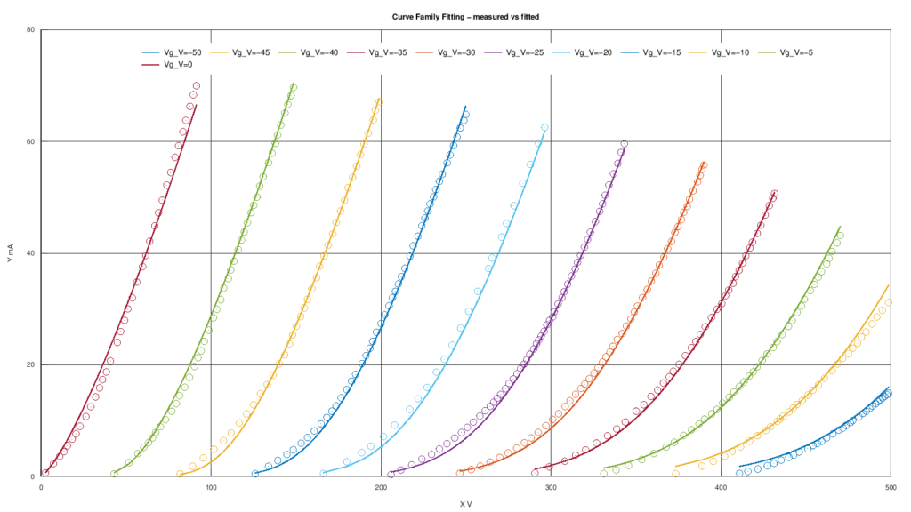
The overlay shows that the model follows the overall family very well but does not pass through every point. That is exactly what should be expected from a compact five-parameter model: a large amount of original information is compressed into one continuous function.

15. Absolute residuals: where the model is wrong

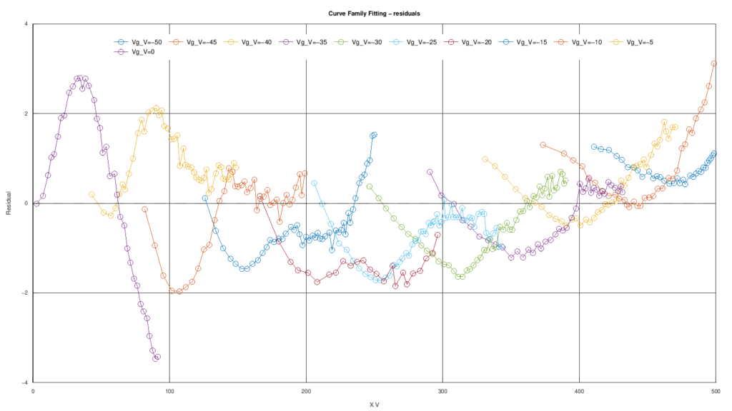
The residuals are not pure random noise. Some families show arcs and sign reversals. This is instructive: the model captures the global surface very well but does not have enough degrees of freedom to reproduce every local detail of the digitized curves.

For studying a compact model, the residual plot is often more informative than the fitted curve itself because it shows exactly what the equation fails to explain.

16. Relative residuals: why they become large near cutoff

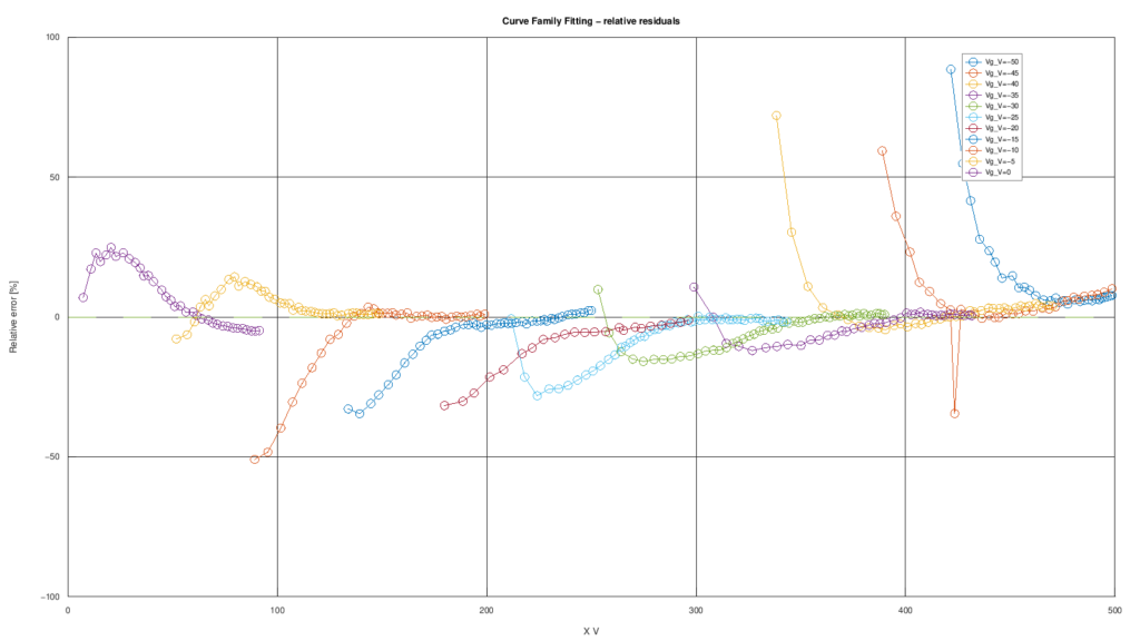
If the reference current is 0.5 mA, an absolute error of only 0.25 mA is already 50%. Large percentage errors near cutoff can therefore coexist with small absolute residuals.

This plot should be read together with the residual plot in mA, not instead of it. One describes absolute current error; the other shows how large that error is relative to the local current.

17. Parity plot: excellent globally, poor at locating the error

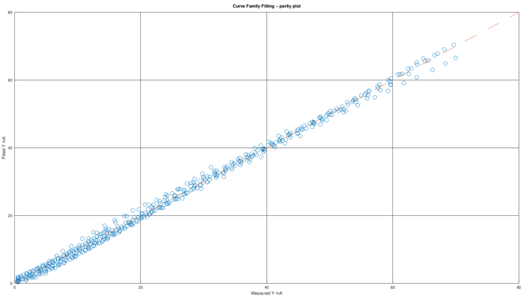
The parity plot removes \(V_{ak}\) and \(V_{gk}\) and compares predicted current directly with reference current. It is excellent for global bias, scatter, and outliers, but it cannot show which curve family or voltage region is responsible. It therefore cannot replace residual plots.

18. Error by family

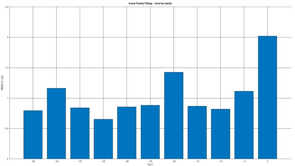
Different family RMSE values are another indication of structural model limitations. They do not automatically mean that the worse curves were digitized less accurately. A five-parameter function may simply be unable to match every part of the real surface equally well.

19. Training domain: the min/max rectangle is misleading

Stating that the dataset runs from 2.73 to 498.63 V and from -50 to 0 V does not mean that data exist everywhere inside that rectangle. Different grid-voltage families cover different plate-voltage intervals. GX-TXT therefore stores the training domain as the convex hull of the 440 points.

The distinction is essential:

• interpolation: evaluating the model inside a region actually covered by data;
• extrapolation: asking the equation to predict behavior not constrained by those data.

An analytic model will usually return a perfectly smooth number during extrapolation. That is precisely why extrapolation can be dangerous: numerical regularity is not evidence of physical validity.

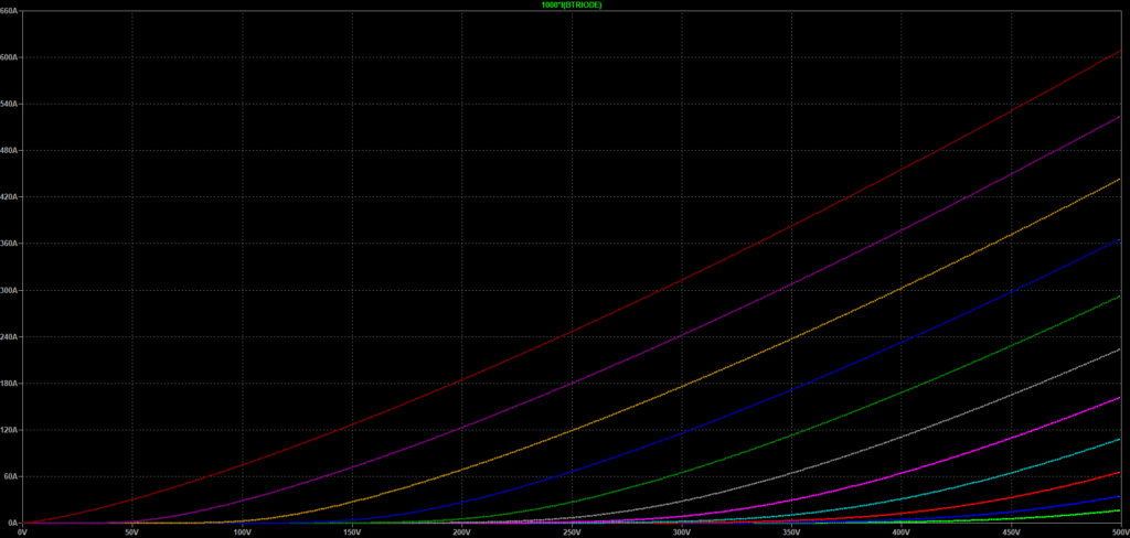
20. The LTspice sweep makes extrapolation visible

To verify the implementation I translated the same equation into an LTspice behavioral current source and ran:

.step param Vgk -50 0 5
.dc VA 0 500 1

The simulator therefore generates eleven complete curves from 0 to 500 V whether or not the original dataset contains points in every region. At 500 V, for example, the LTspice CSV gives:

Vgk [V]	Ia at 500 V [mA]
-50	16.4697
-45	35.0059
-40	65.6325
-35	108.7762
-30	162.6170
-25	224.7502
-20	293.2140
-15	366.6666
-10	444.2369
-5	525.3525
0	609.6198

The important number is not 609.6 mA by itself. The fitting dataset reaches only about 69.99 mA. The equation continues smoothly beyond 600 mA because the mathematical function does not know where the experimental domain ended. This makes the plot a particularly clear illustration of a general rule:

a simulation that converges is not automatically a physically validated simulation.

21. LTspice validation netlist

The netlist reproduces triode_koren_v1 using a behavioral current source. LTspice current is expressed in amperes, so the factor 2000 used by GX-TXT in mA becomes 2.

* 6BX7-GT -- LTspice validation of GX-TXT triode.koren_v1
.param mu=10.813884978151192
.param Kp=77.284607645620596
.param Kvb=654.33045589862036
.param Kg1=485.64217355533503
.param Ex=1.3034825268711401
.param Vgk=-20

.func den(vak)      {sqrt(max(Kvb + vak*vak, 1e-30))}
.func zk(vak,vgk)   {Kp*(1/mu + vgk/den(vak))}
.func softplus(x)    {max(x,0) + ln(1 + exp(-abs(x)))}
.func eone(vak,vgk) {max((vak/Kp)*softplus(zk(vak,vgk)),0)}
.func ia_koren(vak,vgk) {2*pwr(eone(vak,vgk),Ex)/Kg1}

VA A 0 0
VG G 0 {Vgk}
BTRIODE A 0 I=ia_koren(V(A),V(G))

.step param Vgk -50 0 5
.dc VA 0 500 1
.options plotwinsize=0
.end

Download the LTspice validation netlist

Spot checks of the CSV show that LTspice and the Octave implementation return the same values to the displayed precision. For example, at \(V_{ak}=500\) V and \(V_{gk}=-50\) V both give approximately 16.4697 mA; at \(V_{gk}=0\) V both give approximately 609.6198 mA. This validates the translation of the equation, not the physical validity of those extreme operating points.

22. This is not yet a complete 6BX7-GT SPICE macro-model

The B-source is useful for mathematical validation, but it would be misleading to call it a complete tube model. At minimum it lacks:

• inter-electrode capacitances;
• positive-grid current;
• additional elements that may be needed for robust convergence in complex circuits;
• unit spread, temperature effects, and aging.

For DC simulation inside the fitted domain, the behavioral source is exactly what is needed. For transient simulation, frequency response, or positive-grid operation, a more complete subcircuit is required.

23. What I consider trustworthy in this model — and what I do not

Use	Assessment	Reason
Interpolation of static characteristics inside the data-covered domain	Good	Global fit RMSE ≈ 1.07 mA and \(R^2\approx0.9966\).
Qualitative comparison of operating points inside the domain	Good	The surface is continuous and follows the digitized families closely.
Near-cutoff region	Use caution	Relative errors can become large despite small absolute residuals.
Positive grid voltage	Not validated	The dataset stops at 0 V and the validation netlist has no grid-current model.
Currents far above 70 mA	Extrapolation	Outside the reference-current range used for fitting.
Frequency response	Not described by the static equation	Inter-electrode capacitances are absent.
Variation among real tubes	Not described	The fit represents one nominal data family, not a statistical population of devices.

24. What the 6BX7-GT case study teaches about compact models

The most useful result of this work is not simply a set of five numbers to paste into SPICE. The fitting makes the meaning of a model very concrete:

• the Langmuir-Child law provides the physical intuition;
• Koren adds a phenomenological equation that follows real curves much better;
• the nonlinear optimizer determines the parameter set that best represents one dataset;
• residuals expose the behavior that the equation cannot explain;
• the training domain separates interpolation from extrapolation;
• SPICE faithfully evaluates the equation, but cannot know when we are using it outside its validated region.

The last point is the most important. A good model is not one that always produces a number; it is one whose accuracy and limitations are both understood.

25. References

1. Norman L. Koren, Improved vacuum tube models for SPICE simulations, Part 1: Models and example, web version updated 2003: normankoren.com/Audio/Tubemodspice_article.html.
2. Norman L. Koren, Finding SPICE tube model parameters: normankoren.com/Audio/Tube_params.html.
3. Norman L. Koren, Improved vacuum tube models for SPICE simulations, Part 2, including complete subcircuit examples: normankoren.com/Audio/Tubemodspice_article_2.html.
4. General Electric, 6BX7-GT characteristic data used as the source for curve digitization.
5. GX-TXT, curvefit.family_global module, triode.koren_v1 model, global 6BX7-GT fitting session.