OpenFOAM: conjugate heat transfer, interface and stability

25 October 2026 by giux CFD and OpenFOAM, Featured 33 min read

Deep dive linked to Guide 11 — conjugate heat transfer (CHT) of the Learning OpenFOAM 14 path. The article was built by querying a research notebook loaded with the cited sources (open-access papers and reviews, excerpts of the OpenFOAM 14 source and Guide 11), then checking every number against the original sources and the version 14 repository; the one-dimensional model of section 8 was run and its results are reported unchanged. The video at the top summarises the same path.

Deep-dive video: conjugate heat transfer in OpenFOAM 14, interface and stability (generated with Gemini Notebook from the cited sources).

What it is about. This deep dive grows out of Guide 11 and answers a precise question: what happens, numerically, at the interface between a fluid and a solid when OpenFOAM 14 solves the regions one after the other, and how to verify that the result does not depend on the way they are coupled. We start from the conjugate problem in the classical literature, read the coupledTemperature condition and the foamMultiRun loop line by line, reconstruct the stability theory of partitioned methods (Giles, Verstraete and Scholl, Errera, CHAMP), compare monolithic and partitioned coupling with the data of Tandis, Cardiff and Ashrafizadeh (2025) and check everything with an executable one-dimensional model. Every number is taken from the cited sources or computed with the script given in full; where the sources do not say something, we state it.

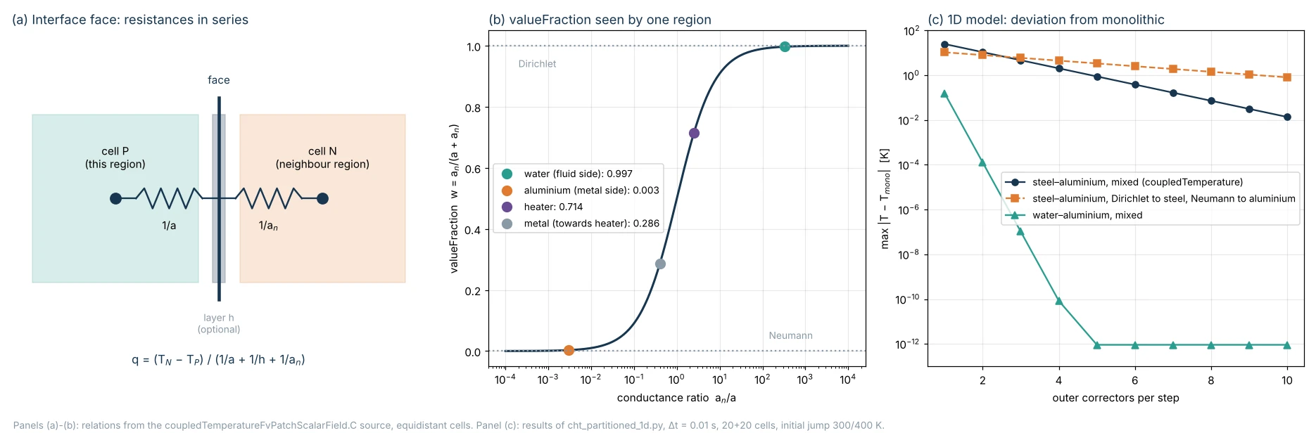
Series resistances at the interface face, coupledTemperature valueFraction for water, aluminium and heater, and deviation from monolithic in the 1D model versus outer correctors — Interface, weights and coupling convergence

1. The conjugate problem and when it is really needed

In most heat transfer computations the wall is described by a boundary condition: imposed temperature, imposed flux, or a heat transfer coefficient h with a reference temperature (third-kind condition). The conjugate problem gives up all three: conduction in the solid and convection in the fluid are solved together, and the interface temperature and flux become results of the computation.

The term originates with T. L. Perelman (1961) and is developed by A. V. Luikov (1974). The open-access review by A. Dorfman and Z. Renner (2009) covers almost two hundred publications and shows with quantitative examples when a constant coefficient h stops working:

comparable resistances. For a metal plate washed by liquid metal, the “usual” method with an isothermal-wall h is off by 15–20 %; in turbulent flow the maximum error reported is about 7 %. The parameter that measures the relative weight of the resistances is a wall Biot number, Bi* = h*Δ/λw, and for two fluids separated by a plate the overall Biot number is 1/BiΣ = 1/Bi*₁ + 1/Bi*₂;
wall temperature varying along the flow. The heat flux depends on the upstream history of the boundary layer, which a local h does not contain;
fins. With N² = h̄H²/(λwΔ) below 2 the usual and conjugate methods agree; as N² grows the error on fin efficiency reaches 60–70 %, and for N² ≥ 1.9 heat-flux inversion appears on the back side;
transients. The quasi-steady solution gives large errors especially for Fo < 0.5; in the review’s example the Laplace-transform analytical solution agrees with the numerical one only up to Fo < 0.35.

The heatedDuct tutorial of Guide 11 belongs to the first and second categories: a highly conductive aluminium wall, heated only from the bottom, spreads the heat around the perimeter of a water channel in laminar flow. A uniform h imposed in advance would give a wrong temperature distribution from the start.

2. Interface conditions: from the continuum to the discrete face

For an ideal interface (perfect contact, no surface sources) two conditions hold:

T_f = T_s                                   temperature continuity
kappa_f dT_f/dn = kappa_s dT_s/dn           normal flux continuity

In a finite-volume discretisation the interface face has a cell P on one side, at distance δP, and a cell N on the other, at distance δN. Patankar (1980, chapter 4, interface conductivity) shows that the face conductivity must be built as resistances in series, not as an arithmetic mean of the conductivities:

q = (T_N - T_P) / (delta_P/kappa_P + delta_N/kappa_N)
kappa_face = 2 kappa_P kappa_N / (kappa_P + kappa_N)        if delta_P = delta_N

The arithmetic mean overestimates the flux when the conductivities differ widely: with water (0.606 W/(m K)) and aluminium (200 W/(m K)) it would be about 100 W/(m K), whereas the harmonic mean is 1.21 W/(m K), twice that of water, which is the physically correct value for two half-cells in series. A monolithic solver treats the interface as an internal face with this conductivity; Tandis et al. (2025) write it as ki = kPkN/((ΔP/Δ)kN + (ΔN/Δ)kP), which is the same expression.

3. `coupledTemperature` line by line

OpenFOAM 14 solves the regions separately, so the interface is not an internal face but a pair of mapped (or mappedWall) patches, one per region, with the coupledTemperature condition on both. In the updateCoeffs() method of coupledTemperatureFvPatchScalarField.C, for each face:

Excerpt from coupledTemperatureFvPatchScalarField.C, OpenFOAM 14, lines 407–481 (GPL v3, The OpenFOAM Foundation):

tmp<scalarField> kappa;
tmp<scalarField> sumKappaTByDelta;
tmp<scalarField> sumKappaByDelta;
tmp<scalarField> qByKappa;

// q = alpha.this*sumq
getThis(kappa, sumKappaTByDelta, sumKappaByDelta, sumq, qByKappa);

// Add neighbour contributions
{
    tmp<scalarField> sumKappaTByDeltaNbr;
    tmp<scalarField> sumKappaByDeltaNbr;
    tmp<scalarField> qNbr;

    coupledTemperatureNbr.getNbr
    (
        sumKappaTByDeltaNbr,
        sumKappaByDeltaNbr,
        qNbr
    );

    // Include the effect of the optional neighbour insulation layer
    if (coupledTemperatureNbr.h_.valid())
    {
        const_cast<coupledTemperatureFvPatchScalarField&>
        (
            coupledTemperatureNbr
        ).h_->update();

        const scalarField hFactor
        (
            coupledTemperatureNbr.h_()
           /(coupledTemperatureNbr.h_() + sumKappaByDeltaNbr())
        );
        sumKappaTByDeltaNbr.ref() *= hFactor;
        sumKappaByDeltaNbr.ref() *= hFactor;
    }

    tmp<scalarField> sumKappaTByDeltaNbrMapped
    (
        mapper.fromNeighbour(sumKappaTByDeltaNbr)
    );

    tmp<scalarField> sumKappaByDeltaNbrMapped
    (
        mapper.fromNeighbour(sumKappaByDeltaNbr)
    );

    // Include the effect of the optional insulation layer
    if (h_.valid())
    {
        h_->update();

        const scalarField hFactor(h_()/(h_() + sumKappaByDeltaNbrMapped()));
        sumKappaTByDeltaNbrMapped.ref() *= hFactor;
        sumKappaByDeltaNbrMapped.ref() *= hFactor;
    }

    add(sumKappaTByDelta, sumKappaTByDeltaNbrMapped);
    add(sumKappaByDelta, sumKappaByDeltaNbrMapped);

    if (qNbr.valid())
    {
        sumq += mapper.fromNeighbour(qNbr);
    }
}

this->valueFraction() =
    sumKappaByDelta()/(kappa()*patch().deltaCoeffs() + sumKappaByDelta());

this->refValue() = (sumKappaTByDelta() + sumq)/sumKappaByDelta();

this->refGrad() = qByKappa;

mixedFvPatchScalarField::updateCoeffs();

In the code a is kappaEff*deltaCoeffs of the cell in this region (κeff taken from the region’s thermophysical transport model: this is why the condition works in both fluids and solids) and a_n is the same quantity of the cell on the other side, brought onto the face by the mapper. A mixed condition assigns the face value Tface = w·refValue + (1 − w)(TP + refGradient/deltaCoeffs). Substituting the three coefficients, without sources:

valueFraction  w = a_n / (a + a_n)
refValue         = (a_n*T_n + q_corr) / a_n
refGradient      = q_s / kappa

T_face = (a*T_P + a_n*T_n) / (a + a_n)
q      = a*a_n/(a + a_n) * (T_n - T_P) = (T_n - T_P) / (1/a + 1/a_n)

This is exactly Patankar’s formula: at convergence the partitioned discretisation coincides with the monolithic one. The difference is in time: Tn is the value the neighbouring region has when the current region is solved, i.e. that of the previous outer iteration or, with a single outer corrector, of the previous time step. In the literature this is a Robin (mixed) condition on both sides, with a coefficient equal to the conductance of the neighbouring cell.

The options, read from the source:

Entry	Meaning	Notes from the code
`Tnbr`	name of the temperature field in the neighbouring region (default `T`)	if the neighbouring patch is not `coupledTemperature` the run stops with a fatal error naming the type found
`h`	resistance of a thin unmeshed layer	`wallLayersHeatTransferCoefficient` function with `thicknessLayers` and `kappaLayers`; the code multiplies the neighbouring conductance by h/(h + a<sub>n</sub>), i.e. adds 1/h in series, with h = 1/Σ(t<sub>i</sub>/κ<sub>i</sub>)
`qs`, `Qs`	source flux on the interface (W/m²) or total power (W)	`Qs` is divided by the patch area; specifying both is a fatal error
`qr`, `qrNbr`, `qrRelaxation`	radiative flux of this region or of the neighbour	added to the balance with relaxation (default 1); used by `vacuumFurnace` and `reverseBurner`
historical names	`compressible::turbulentTemperatureCoupledBaffleMixed`, `compressible::turbulentTemperatureRadCoupledMixed`	registered as aliases and read as `coupledTemperature`

Example of a contact layer, in the style of the thermalBending tutorial (where it is present but commented out):

interface_to_metal
{
    type            coupledTemperature;
    h
    {
        type            wallLayersHeatTransferCoefficient;
        thicknessLayers (1e-4);       // 0.1 mm of thermal paste
        kappaLayers     (1.0);        // W/(m K)
    }
    value           $internalField;
}

With these values h = 1/(10⁻⁴/1) = 10⁴ W/(m² K); an aluminium cell 1 mm from the face has a = 200/0.001 = 2·10⁵ W/(m² K): the layer dominates the resistance on the metal side by a factor of 20.

A detail that can only be read in the code: in updateCoeffs() the conductance of the neighbouring cell is multiplied both by the factor of the neighbouring patch’s h layer and by that of the current patch. The resistances defined on the two patches therefore add up in series: a single physical layer (a thermal paste, a gap) must be defined on only one of the two patches, otherwise its resistance counts twice. The thermalBending tutorial has, commented out, one layer per side (1 µm on the heat sink and 10 µm on the plate, both with κ = 0.025): if activated, the total resistance is that of 11 µm.

Two pedantic remarks on the version 14 source. The header of the .H file still describes thicknessLayers and kappaLayers entries directly in the patch, whereas the code reads them only inside the h subdictionary. And qs is read with declared dimensions dimPower/dimTime instead of W/m², so it is best written as a plain number without explicit units; the “Usage” table of the documentation correctly states W/m².

4. The weights in the `heatedDuct` case

With the tutorial properties (water κ = μcp/Pr = 959·10⁻⁶ × 4181/6.62 ≈ 0.606 W/(m K), aluminium 200, heater 80) and cells at the same distance from the face, the weights are those of panel (b) of the figure:

Interface	Region	valueFraction	What it receives
fluid–metal	`fluid`	200/200.6 ≈ 0.997	practically the metal temperature (almost Dirichlet)
fluid–metal	`metal`	0.606/200.6 ≈ 0.003	practically the flux from the fluid (almost Neumann)
metal–heater	`heater`	200/280 ≈ 0.714	mixed condition
metal–heater	`metal`	80/280 ≈ 0.286	mixed condition

On the fluid-metal interface the condition reduces by itself to the scheme the theory (section 6) recommends: Dirichlet to the fluid, Neumann to the solid. On the interface between two solids of comparable conductivity the weights are intermediate and the coupling is stronger. With different distances the weight follows the ratio an/a = (κn/δn)/(κ/δ): a fluid cell squeezed against the wall (prism layers) increases a and shifts the weight towards the fluid, without changing the nature of the result as long as the conductivity ratio remains two orders of magnitude.

5. The `foamMultiRun` loop

foamMultiRun loads one module per region (regionSolvers entry of controlDict: in heatedDuct fluid fluid; metal solid; heater solid;) and advances them together. In foamMultiRun.C, at every time step and for every outer corrector, each phase is executed on all regions before moving to the next:

for each outer corrector (nOuterCorrectors):
    moveMesh, motionCorrector             regions with motion
    fvModels().correct()
    prePredictor
    momentumTransportPredictor            fluids
    thermophysicalTransportPredictor
    momentumPredictor                     fluids
    while (pimple.correctEnergy())        nEnergyCorrectors, default 1
        thermophysicalPredictor           energy of ALL regions, in order
    pressureCorrector                     fluids
    momentumTransportCorrector, thermophysicalTransportCorrector

There are therefore three levers, with different roles:

nEnergyCorrectors, in the top-level PIMPLE (system/fvSolution, read by pimpleMultiRegionControl.C): repeats only the energy equations of all regions, exchanging the interface temperatures at each pass, without solving momentum and pressure again. It is the cheapest lever when the flow does not depend on temperature; VoFcoolingCylinder2D uses 2;
nOuterCorrectors, in the same block: repeats the whole sequence; needed when temperature acts on the flow (buoyancy, variable properties). engine2Valve2D and multiphaseCoolingCylinder2D use 3;
outerCorrectorResidualControl, in the PIMPLE of each region: stops the outer correctors when the initial residuals fall below tolerance and relTol (both mandatory: otherwise a fatal error). It is used with nOuterCorrectors greater than 1 as an upper bound. For steady computations residualControl stops the run: circuitBoardCooling uses it with e 1e-4 in the solid and U, h 1e-4 in the fluid.

The time step is the minimum of the regions’ maxDeltaT() (setDeltaT.C): in the fluid basicFluidSolver.C combines maxDeltaT and maxCo; in the solid solid.C only uses maxDeltaT from controlDict and the fvModels limits, without any diffusion-number limit. The step can grow by at most solver::deltaTFactor times from one step to the next. In heatedDuct the top-level PIMPLE block is empty: one outer corrector and one energy corrector, i.e. interface exchange lagged by one step.

6. Stability theory: Giles (1997)

M. B. Giles analysed with the normal-mode method a one-dimensional model problem: two materials with constant coefficients, interface at x = 0, uniform grids Δx₋ and Δx₊, finite-volume discretisation. The parameters are the cell Fourier number on each side, d = κΔt/(cΔx²), with c the volumetric heat capacity, and the capacity ratio of the adjacent cells, r = c₊Δx₊/(c₋Δx₋). The − side (solid) receives the flux from the other side, the + side (fluid) receives the temperature: for this choice r = cfΔxf/(csΔxs).

Scheme	Stability condition	Numerical check in the paper
coupled in a single system, explicit	d₋, d₊ ≤ 1/2 (maximum principle)	—
coupled in a single system, implicit	unconditionally stable	—
partitioned explicit	r < √(1 − 2d₋)/(1 − √(1 − 2d₊)) (eq. 4.17)	d₋ = d₊ = 3/8: limit r < 1; r = 0.99 stable, r = 1.01 unstable
hybrid (solid implicit, fluid explicit)	r < √(1 + 2d₋)/(1 − √(1 − 2d₊)) (eq. 4.30)	d₋ = 4, d₊ = 3/8: limit r < 6; r = 5.95 stable, r = 6.05 unstable
partitioned implicit, interface data lagged by one step	for d₋, d₊ ≫ 1: r < √(d₋/d₊) (eq. 4.44)	d₋ = d₊ = 50: limit r < 1; r = 1 stable, r = 1.1 unstable

The instability, when present, is a sawtooth mode at the interface. The paper’s conclusion is clear: the key to stability is to give the structural computation a Neumann condition and the fluid a Dirichlet condition; the reverse scheme is unstable except for very small steps. For gases and metals r is tiny, because the volumetric capacity of a gas is three orders of magnitude smaller.

The partitioned implicit case is that of foamMultiRun with a single outer corrector. Applied to water and aluminium with equal cells: r = 4.18·10⁶/2.43·10⁶ ≈ 1.72 and √(ds/df) = √(αs/αf) = √(8.23·10⁻⁵/1.449·10⁻⁷) ≈ 23.8. The recommended scheme is stable with a wide margin. The reverse scheme (Neumann to water, Dirichlet to aluminium) swaps the roles: r′ = 2.43/4.18 ≈ 0.58 against a limit √(αf/αs) ≈ 0.042, hence unstable. Section 8 checks both predictions.

Giles does not treat mixed conditions: he only considers Dirichlet and Neumann. The next step of the literature is precisely this.

7. After Giles: Biot, optimal Robin conditions, CHAMP

T. Verstraete, S. Scholl (2016) compare three established partitioned methods, propose a fourth and derive a closed-form stability criterion in which the dominant parameter is the Biot number: each method has its own range of applicability and the new one is more stable especially at high Biot.
M.-P. Errera, S. Chemin (2013) derive, again with normal modes, the optimal coefficients of the Robin interface conditions; the line continues with Errera and Duchaine (2016) on the Dirichlet-Robin procedure and with Moretti, Errera, Couaillier and Feyel (2018) on weak and strong coupling.
F. Meng, J. W. Banks, W. D. Henshaw, D. W. Schwendeman (2017), CHAMP scheme: generalised Robin condition with weights chosen by optimising stability; stable and second order with a single implicit solve per domain per step in most cases, with sub-iterations only in extreme cases (very fine grids and large steps). The authors report that it outperforms Dirichlet-Neumann when conductivities and diffusivities differ.

The OpenFOAM condition is a Robin-Robin one with a specific coefficient, the conductance of the neighbouring cell: it is not optimised in the sense of Errera or CHAMP, but it has two useful properties. At convergence it coincides with Patankar’s monolithic discretisation; and, when the conductivities differ widely, it automatically degenerates into the Dirichlet-fluid/Neumann-solid choice that Giles recommends.

8. An executable check: the one-dimensional model

To see all this in numbers, the following script solves transient conduction in two adjacent slabs (5 mm each, 20 cells per side, implicit Euler), with temperature imposed at the outer ends and an initial 300/400 K jump. It compares the monolithic solution with three partitioned couplings solved in sequence (first A, then B) with nOuter correctors per step: the mixed coupledTemperature condition, Dirichlet to A and Neumann to B (DN), and the reverse (ND). It only needs numpy and writes no files.

#!/usr/bin/env python3
"""1D two-material transient conduction: monolithic versus partitioned coupling.

Region A (x < 0) and region B (x > 0), uniform cells, implicit Euler in each region.
Interface treatments:
  mono   : single linear system, face conductance 1/(1/a_A + 1/a_B)  (Patankar)
  mixed  : OpenFOAM coupledTemperature style; each region sees
           T_face = (a_self*T_P + a_nbr*T_nbr)/(a_self + a_nbr) with T_nbr lagged
  DN     : Dirichlet to A (face T from B), Neumann to B (flux from A)
  ND     : the reverse: Neumann to A, Dirichlet to B
With many outer correctors every partitioned scheme that converges reproduces the
monolithic solution to round-off (check with --outer 200).
Regions are solved one after the other (A then B) inside nOuter correctors per step.
Prints the maximum deviation from the monolithic solution and the interface flux.
Only numpy is required. Nothing is written to disk.
"""
import argparse
import numpy as np


def tridiag(lo, di, up, rhs):
    n = len(di); c = np.zeros(n); d = np.zeros(n)
    c[0] = up[0] / di[0]; d[0] = rhs[0] / di[0]
    for i in range(1, n):
        m = di[i] - lo[i] * c[i - 1]
        c[i] = up[i] / m if i < n - 1 else 0.0
        d[i] = (rhs[i] - lo[i] * d[i - 1]) / m
    x = np.zeros(n); x[-1] = d[-1]
    for i in range(n - 2, -1, -1):
        x[i] = d[i] - c[i] * x[i + 1]
    return x


def region_system(T_old, k, rc, dx, dt, left, right):
    """Implicit Euler for one region. left/right = ('T', value) Dirichlet at face,
    ('q', flux into region) Neumann, or ('R', a_ext, T_ext) Robin (series conductance)."""
    n = len(T_old); a = k / dx; cap = rc * dx / dt
    lo = np.zeros(n); di = np.full(n, cap); up = np.zeros(n); rhs = cap * T_old.copy()
    for i in range(n):
        if i > 0:
            di[i] += a; lo[i] = -a
        if i < n - 1:
            di[i] += a; up[i] = -a
    for side, bc, idx in (('L', left, 0), ('R', right, n - 1)):
        ab = 2 * k / dx  # centre-to-face conductance
        if bc[0] == 'T':
            di[idx] += ab; rhs[idx] += ab * bc[1]
        elif bc[0] == 'q':
            rhs[idx] += bc[1]
        elif bc[0] == 'R':
            g = 1.0 / (1.0 / ab + 1.0 / bc[1])
            di[idx] += g; rhs[idx] += g * bc[2]
    return tridiag(lo, di, up, rhs)


def run(kA, rcA, kB, rcB, nA, nB, L, dt, steps, scheme, nOuter, T0A=300.0, T0B=400.0, TendA=300.0, TendB=400.0):
    dxA = L / nA; dxB = L / nB
    TA = np.full(nA, T0A); TB = np.full(nB, T0B)
    aA = 2 * kA / dxA; aB = 2 * kB / dxB
    hist = []
    g0 = 1.0 / (1.0 / aA + 1.0 / aB)
    qA = g0 * (T0B - T0A); qB = -qA  # initial interface flux guess (into A, into B)
    for s in range(steps):
        TA_old, TB_old = TA.copy(), TB.copy()
        if scheme == 'mono':
            n = nA + nB; T_old = np.concatenate([TA_old, TB_old])
            k = np.r_[np.full(nA, kA), np.full(nB, kB)]; dx = np.r_[np.full(nA, dxA), np.full(nB, dxB)]
            rc = np.r_[np.full(nA, rcA), np.full(nB, rcB)]
            cap = rc * dx / dt; lo = np.zeros(n); di = cap.copy(); up = np.zeros(n); rhs = cap * T_old
            for i in range(n - 1):
                g = 1.0 / (dx[i] / (2 * k[i]) + dx[i + 1] / (2 * k[i + 1]))
                di[i] += g; up[i] = -g; di[i + 1] += g; lo[i + 1] = -g
            di[0] += aA; rhs[0] += aA * TendA; di[-1] += aB; rhs[-1] += aB * TendB
            T = tridiag(lo, di, up, rhs); TA, TB = T[:nA], T[nA:]
        else:
            for _ in range(nOuter):
                if scheme == 'mixed':
                    TA = region_system(TA_old, kA, rcA, dxA, dt, ('T', TendA), ('R', aB, TB[0]))
                    TB = region_system(TB_old, kB, rcB, dxB, dt, ('R', aA, TA[-1]), ('T', TendB))
                elif scheme == 'DN':
                    # A gets the face temperature of B, B gets the flux computed by A
                    Tf = TB[0] + qB / aB          # face value seen from B (lagged)
                    TA = region_system(TA_old, kA, rcA, dxA, dt, ('T', TendA), ('T', Tf))
                    qA = aA * (Tf - TA[-1])       # flux from the face into A
                    qB = -qA                      # flux from the face into B
                    TB = region_system(TB_old, kB, rcB, dxB, dt, ('q', qB), ('T', TendB))
                elif scheme == 'ND':
                    # A gets the flux computed by B, B gets the face temperature of A
                    TA = region_system(TA_old, kA, rcA, dxA, dt, ('T', TendA), ('q', qA))
                    Tf = TA[-1] + qA / aA         # face value seen from A
                    TB = region_system(TB_old, kB, rcB, dxB, dt, ('T', Tf), ('T', TendB))
                    qB = aB * (Tf - TB[0])        # flux from the face into B
                    qA = -qB
        g = 1.0 / (1.0 / aA + 1.0 / aB)
        hist.append((np.concatenate([TA, TB]), g * (TB[0] - TA[-1])))
    return hist


def main():
    np.seterr(all='ignore')  # the unstable schemes overflow on purpose
    p = argparse.ArgumentParser(description=__doc__, formatter_class=argparse.RawDescriptionHelpFormatter)
    p.add_argument('--pair', choices=['water-aluminium', 'steel-aluminium'], default='water-aluminium',
                   help='region A - region B (A is the first, lower-effusivity material)')
    p.add_argument('--cells', type=int, default=20, help='cells per region')
    p.add_argument('--L', type=float, default=5e-3, help='thickness of each region [m]')
    p.add_argument('--steps', type=int, default=40, help='time steps')
    p.add_argument('--dt', type=float, nargs='+', default=[1e-3, 1e-2, 1e-1, 1.0])
    p.add_argument('--outer', type=int, nargs='+', default=[1, 3, 10])
    a = p.parse_args()
    water = (0.6057, 1000 * 4181); alu = (200.0, 2700 * 900); steel = (80.0, 8000 * 450)
    A, B = (water, alu) if a.pair == 'water-aluminium' else (steel, alu)
    dx = a.L / a.cells
    eA = (A[0] * A[1]) ** 0.5; eB = (B[0] * B[1]) ** 0.5
    print(f'pair {a.pair}: kA={A[0]} rhocA={A[1]:.4g}  kB={B[0]} rhocB={B[1]:.4g}  '
          f'{a.cells}+{a.cells} cells, dx={dx:.3e} m, {a.steps} steps, initial jump 300/400 K')
    print(f'effusivities A={eA:.0f} B={eB:.0f} W s^0.5/(m2 K), sigma={min(eA, eB) / max(eA, eB):.3f}, '
          f'valueFraction seen by A = {B[0] / (A[0] + B[0]):.4f}, by B = {A[0] / (A[0] + B[0]):.4f}')
    print('max|T - T_mono| over all cells and steps [K]; in brackets the value at the last step')
    for dt in a.dt:
        dA = A[0] / A[1] * dt / dx ** 2; dB = B[0] / B[1] * dt / dx ** 2
        ref = run(A[0], A[1], B[0], B[1], a.cells, a.cells, a.L, dt, a.steps, 'mono', 1)
        print(f'dt={dt:g} s  Fourier dA={dA:.3g} dB={dB:.3g}')
        for sch in ('mixed', 'DN', 'ND'):
            line = f'   {sch:5s}'
            for no in a.outer:
                h = run(A[0], A[1], B[0], B[1], a.cells, a.cells, a.L, dt, a.steps, sch, no)
                e = [np.max(np.abs(x[0] - r[0])) for x, r in zip(h, ref)]
                emax = max(e)
                if not np.isfinite(emax) or emax > 1e4:
                    line += f'  nOuter={no:<3d} unstable          '
                else:
                    line += f'  nOuter={no:<3d} {emax:9.3g} [{e[-1]:8.2g}]'
            print(line)


if __name__ == '__main__':
    main()

Water (A)–aluminium (B) pair, σ ≈ 0.072:

pair water-aluminium: kA=0.6057 rhocA=4.181e+06  kB=200.0 rhocB=2.43e+06  20+20 cells, dx=2.500e-04 m, 40 steps, initial jump 300/400 K
effusivities A=1591 B=22045 W s^0.5/(m2 K), sigma=0.072, valueFraction seen by A = 0.9970, by B = 0.0030
max|T - T_mono| over all cells and steps [K]; in brackets the value at the last step
dt=0.001 s  Fourier dA=0.00232 dB=1.32
   mixed  nOuter=1      0.0154 [   0.015]  nOuter=3    6.93e-12 [ 6.9e-12]  nOuter=10   5.17e-12 [ 5.2e-12]
   DN     nOuter=1      0.0146 [   0.015]  nOuter=3    8.37e-07 [ 8.4e-07]  nOuter=10    5.4e-12 [ 5.4e-12]
   ND     nOuter=1   unstable            nOuter=3   unstable            nOuter=10  unstable          
dt=0.01 s  Fourier dA=0.0232 dB=13.2
   mixed  nOuter=1       0.158 [    0.03]  nOuter=3    1.04e-07 [   2e-08]  nOuter=10   9.09e-13 [ 6.8e-13]
   DN     nOuter=1       0.148 [   0.025]  nOuter=3    6.77e-05 [ 1.2e-05]  nOuter=10   8.53e-13 [ 8.5e-13]
   ND     nOuter=1   unstable            nOuter=3   unstable            nOuter=10  unstable          
dt=0.1 s  Fourier dA=0.232 dB=132
   mixed  nOuter=1         1.2 [   0.017]  nOuter=3     0.00032 [ 4.5e-06]  nOuter=10   1.71e-12 [ 1.5e-12]
   DN     nOuter=1        1.17 [   0.016]  nOuter=3     0.00261 [ 3.7e-05]  nOuter=10   1.48e-12 [ 6.8e-13]
   ND     nOuter=1   unstable            nOuter=3   unstable            nOuter=10  unstable          
dt=1 s  Fourier dA=2.32 dB=1.32e+03
   mixed  nOuter=1        2.22 [  0.0046]  nOuter=3     0.00978 [ 1.9e-05]  nOuter=10   5.46e-11 [ 1.2e-12]
   DN     nOuter=1        2.08 [  0.0049]  nOuter=3     0.00246 [   6e-06]  nOuter=10   1.14e-12 [ 6.8e-13]
   ND     nOuter=1   unstable            nOuter=3   unstable            nOuter=10  unstable

Heater steel (A)–aluminium (B) pair, σ ≈ 0.770:

pair steel-aluminium: kA=80.0 rhocA=3.6e+06  kB=200.0 rhocB=2.43e+06  20+20 cells, dx=2.500e-04 m, 40 steps, initial jump 300/400 K
effusivities A=16971 B=22045 W s^0.5/(m2 K), sigma=0.770, valueFraction seen by A = 0.7143, by B = 0.2857
max|T - T_mono| over all cells and steps [K]; in brackets the value at the last step
dt=0.001 s  Fourier dA=0.356 dB=1.32
   mixed  nOuter=1        6.89 [     1.5]  nOuter=3       0.051 [  0.0098]  nOuter=10    1.7e-09 [ 3.3e-10]
   DN     nOuter=1        4.09 [   0.052]  nOuter=3        1.69 [   0.028]  nOuter=10     0.0773 [  0.0016]
   ND     nOuter=1   unstable            nOuter=3   unstable            nOuter=10  unstable          
dt=0.01 s  Fourier dA=3.56 dB=13.2
   mixed  nOuter=1          25 [     1.7]  nOuter=3        4.71 [    0.16]  nOuter=10     0.0137 [  0.0004]
   DN     nOuter=1        10.7 [    0.11]  nOuter=3        6.01 [   0.075]  nOuter=10       0.81 [   0.015]
   ND     nOuter=1   unstable            nOuter=3   unstable            nOuter=10  unstable          
dt=0.1 s  Fourier dA=35.6 dB=132
   mixed  nOuter=1        35.5 [    0.35]  nOuter=3        20.4 [ 0.00059]  nOuter=10       2.93 [   2e-05]
   DN     nOuter=1        12.3 [  0.0003]  nOuter=3        6.44 [ 3.5e-05]  nOuter=10      0.671 [ 4.3e-06]
   ND     nOuter=1   unstable            nOuter=3   unstable            nOuter=10  unstable          
dt=1 s  Fourier dA=356 dB=1.32e+03
   mixed  nOuter=1        30.5 [    0.25]  nOuter=3          23 [ 2.5e-05]  nOuter=10        8.5 [ 2.4e-12]
   DN     nOuter=1         5.3 [ 7.3e-09]  nOuter=3        1.02 [   1e-12]  nOuter=10    0.00698 [ 1.1e-12]
   ND     nOuter=1   unstable            nOuter=3   unstable            nOuter=10  unstable

Consistency check with many correctors (Δt = 0.1 s):

pair water-aluminium: kA=0.6057 rhocA=4.181e+06  kB=200.0 rhocB=2.43e+06  20+20 cells, dx=2.500e-04 m, 40 steps, initial jump 300/400 K
effusivities A=1591 B=22045 W s^0.5/(m2 K), sigma=0.072, valueFraction seen by A = 0.9970, by B = 0.0030
max|T - T_mono| over all cells and steps [K]; in brackets the value at the last step
dt=0.1 s  Fourier dA=0.232 dB=132
   mixed  nOuter=50   1.71e-12 [ 1.5e-12]  nOuter=200  1.71e-12 [ 1.5e-12]
   DN     nOuter=50   8.53e-13 [ 6.8e-13]  nOuter=200  8.53e-13 [ 6.8e-13]
   ND     nOuter=50  unstable            nOuter=200 unstable          
pair steel-aluminium: kA=80.0 rhocA=3.6e+06  kB=200.0 rhocB=2.43e+06  20+20 cells, dx=2.500e-04 m, 40 steps, initial jump 300/400 K
effusivities A=16971 B=22045 W s^0.5/(m2 K), sigma=0.770, valueFraction seen by A = 0.7143, by B = 0.2857
max|T - T_mono| over all cells and steps [K]; in brackets the value at the last step
dt=0.1 s  Fourier dA=35.6 dB=132
   mixed  nOuter=50   4.45e-05 [ 2.4e-10]  nOuter=200  1.25e-12 [ 9.1e-13]
   DN     nOuter=50   1.64e-06 [ 9.4e-12]  nOuter=200  1.93e-12 [   8e-13]
   ND     nOuter=50  unstable            nOuter=200 unstable

What the numbers show:

All the schemes that converge reproduce the monolithic solution to round-off (10⁻¹² K with 200 correctors): partitioned coupling changes the path, not the solution.
The ND scheme is unstable in every case, as Giles predicts: for water-aluminium r′ ≈ 0.58 against a limit ≈ 0.042; for steel-aluminium, with the steel side receiving the flux, r′ = 2.43/3.60 ≈ 0.68 against √(dsteel/daluminium) = √(0.356/1.32) ≈ 0.52.
With small σ (water-aluminium) the mixed condition and DN are almost indistinguishable, because w ≈ 0.997 and 0.003 make them in practice the same scheme; with a single corrector the maximum deviation, due to the first steps after the initial jump, ranges from 0.015 K (Δt = 1 ms) to 2.2 K (Δt = 1 s), and at the last step it stays within 0.03 K. Three correctors are enough to reach 10⁻² K even with Δt = 1 s.
With σ ≈ 0.77 (steel-aluminium) the coupling is strong: with the mixed condition and a single corrector the maximum deviation reaches 25–35 K on a 100 K jump for Δt ≥ 0.01 s. With Δt = 0.01 s the mixed condition converges faster than DN (factor ≈ 0.43 per corrector against ≈ 0.75: panel (c) of the figure), while with very large steps (Δt = 1 s, d ≫ 1) DN converges faster. Neither scheme is best in absolute terms: it is the same conclusion, with other parameters, as Verstraete and Scholl and the Errera line of work.

The model is one-dimensional and without convection: it does not replace a three-dimensional case, but it isolates exactly the interface mechanism and allows the effect of step, correctors and properties to be checked in a few seconds.

9. Monolithic versus partitioned in OpenFOAM: Tandis, Cardiff and Ashrafizadeh (2025)

The reference closest to this article is E. Tandis, P. Cardiff, A. Ashrafizadeh, “Analysis of Coupling Strategies for Conjugate Heat Transfer Problems”, OpenFOAM® Journal 5 (2025) 38–58, open access (CC BY-SA 4.0). The authors review the CHT solvers of foam-extend 4.0 (conjugateHeatFoam, monolithic, one fluid and one solid region, Boussinesq; chtMultiRegionFoam, partitioned), of OpenFOAM-v2112 and of OpenFOAM-9, describe the mixed condition of the partitioned solvers with the same weight ω = (kN/ΔN)/(kP/ΔP + kN/ΔN) as section 3 and propose a single solver (multiChtFoam) with three algorithms: classic partitioned with an integrated loop (SIPM-IP, like chtMultiRegionFoam), partitioned with a separate loop for the interface (SIPM-SP) and multi-region monolithic (SIPM-M).

The strength of the thermal coupling is measured by the effusivity ratio σ = (k₁/√α₁)/(k₂/√α₂), with the region of larger effusivity in the denominator, hence 0 < σ < 1; σ → 1 means that both regions vary strongly and the temperature-temperature coupling is strong. The Grashof number instead measures the pressure-velocity-temperature coupling. The test case is a 1 m square cavity with a 0.2 m solid wall (80×80 cells in the fluid, 80×20 in the solid, Δt = 2.5·10⁻⁴ s, Pr = 0.7):

State	k<sub>s</sub>/k<sub>f</sub>	Gr	σ	Outer iterations IP / SP / M	CPU IP / SP / M [s]
A	1.6	1.43·10⁵	0.93	12.2 / 9.3 / 9.3	40.1 / 32.3 / 30.17
B	1.6	10⁴	0.93	12.7 / 5.6 / 5.6	41.7 / 22.9 / 20.79
C	1600	1.43·10⁵	4·10⁻⁴	10.3 / 9.3 / 8.7	36.5 / 30.6 / 28.8
D	1600	10⁴	4·10⁻⁴	7.5 / 5.5 / 5.4	29.0 / 21.2 / 20.43

With the momentum predictor on, the monolithic approach costs 21 to 50 % less than the classic partitioned one; with three cavities and three walls (same states) the advantage grows: in state B 137.2 s for IP against 69.3 s for M (15.6 against 6.6 outer iterations). The authors conclude that enforcing the interface conditions with a dedicated inner loop or a simultaneous solve can speed up the computation up to two times, and that the monolithic approach is superior especially with more than two regions. In OpenFOAM 14 the closest equivalent of the separate loop is nEnergyCorrectors, which repeats only the energy: it is the first thing to try when the interface exchange is the bottleneck.

10. Effusivity and coupling strength in `heatedDuct`

The effusivities e = √(κρc) of the three regions, already computed by the cht_estimates.py script of Guide 11, are 1591 (water), 22045 (aluminium) and 16971 (heater) W s0.5/(m² K). Hence:

Interface	σ	Coupling	Practical consequence
water–aluminium	1591/22045 ≈ 0.072	weak	the one-step lag matters little; the main check is the mesh on the fluid side, where all the resistance is
heater–aluminium	16971/22045 ≈ 0.77	strong	it is the interface most sensitive to the correctors: the Q(metal_to_heater) + Q(heater_to_metal) ≈ 0 balance of section 13 of the guide must be checked first

The picture is consistent with the weights of section 4 and with the 1D model of section 8: where σ is small the interface behaves as Dirichlet-Neumann and converges in a few correctors, where σ is close to 1 more correctors or smaller steps are needed.

11. Reference values for the square duct

For fully developed laminar flow in a square duct, Shah and London (1978) report, with Dh as the reference length:

Quantity	Value	Thermal wall condition
f·Re (Fanning)	14.227 (Darcy 56.91)	—
Nu<sub>T</sub>	2.976	temperature uniform over perimeter and length
Nu<sub>H1</sub>	3.608	axially uniform flux, peripherally uniform temperature (highly conductive wall)
Nu<sub>H2</sub>	3.091	flux uniform around the perimeter too (wall without circumferential conduction)

The same rounded values (2.98 and 3.61) are tabulated by Muzychka and Yovanovich (2002, open access). The distinction between H1 and H2 is a conjugate effect: a highly conductive aluminium wall brings heatedDuct close to the H1 condition even though heat enters only from the bottom; lowering the metal κ (the steel exercise of Guide 11) moves towards H2 and the mean Nusselt number decreases.

Neither value is compared directly with the tutorial: with Re ≈ 42 and Pr = 6.62 the thermal entry length estimated with 0.05 Re Pr Dh is about 0.55 m, 3.7 times the 0.15 m duct; at t = 20 s the case is still a transient, with a flow-through time L/U = 150 s and an overall time constant of about 227 s. A quantitative comparison would require a steady copy with a much longer duct, reduced power and a Nusselt number defined from the mixed-mean temperature and the mean wall temperature.

12. Frozen flow: steady state without solving the flow

The vacuumFurnace tutorial (50 kW heater, radiation and natural convection) accelerates the cooling of a steel block with three strategies described in its README: frozen (flow computed once, then energy only), periodic (flow recomputed at intervals) and continuous. Its Allrun sets PIMPLE/flow to off in system/fluid/fvSolution with foamDictionary and raises the step from 0.05 s to 50 s.

In heatedDuct the same technique is exact: zero gravity and constant density and viscosity make the momentum independent of temperature. In a new copy, after the flow field has reached steady state:

foamDictionary system/fluid/fvSolution -entry PIMPLE/flow -set off
foamDictionary system/controlDict -set "adjustTimeStep=no, deltaT=1, endTime=2000"
foamMultiRun > log.foamMultiRun.frozen 2>&1

adjustTimeStep must be disabled: even with frozen flow, basicFluidSolver::maxDeltaT() keeps limiting the step with maxCo computed on the existing phi flux. The useful result is the steady state; the time history obtained with large steps is not accurate and must not be used as a transient.

13. A verification protocol for `heatedDuct`

Every test is run in a new copy of the case, recording the change, as in Guide 11.

Reference. The tutorial case, with the guide’s measurements: maximum temperatures per region, interface powers (wallHeatFlux), outlet mixed-mean temperature, balance with storage.
Energy correctors. nEnergyCorrectors 3 in the top-level PIMPLE. If the interface powers change beyond the tolerance, the thermal coupling was not converged.
Outer correctors with residual control. nOuterCorrectors 10 with outerCorrectorResidualControl in every region: the log shows how many correctors each step really needs.
Step. Halved maxDeltaT: do the solid temperatures change? In the solid there is no automatic limit on the Fourier number.
Conservation. Q(fluid_to_metal) + Q(metal_to_fluid) ≈ 0 and Q(metal_to_heater) + Q(heater_to_metal) ≈ 0 at every saved time, with the sum compared with the powers involved: a systematic offset indicates a patch-mapping problem or a non-converged coupling.
Fluid-side mesh. That is where the resistance is: refining near the wall weighs on the exchanged flux more than any other parameter.

// system/fvSolution (top level), copy "ecorr3"
PIMPLE
{
    nEnergyCorrectors  3;
}

// system/fvSolution (top level), copy "outer10"
PIMPLE
{
    nOuterCorrectors   10;
}
// and in system/fluid/fvSolution, system/metal/fvSolution, system/heater/fvSolution
PIMPLE
{
    outerCorrectorResidualControl
    {
        "h|e"  { tolerance 1e-6; relTol 0; }
    }
}

14. The other OpenFOAM 14 CHT tutorials

Tutorial	Regions → modules	Time and correctors	What it shows
`coolingCylinder2D`	fluid → fluid, solid → solid	Euler, fixed Δt 0.01 s, 1 corrector	the minimal case: `blockMesh`, `splitMeshRegions -cellZones`, `foamMultiRun`
`VoFcoolingCylinder2D`	fluid → compressibleVoF, solid → solid	maxCo 2, `nEnergyCorrectors 2`	CHT with a two-phase free-surface fluid
`multiphaseCoolingCylinder2D`	fluid → multiphaseEuler, solid → solid	maxCo 0.25, 3 correctors	CHT with the Eulerian multiphase model
`wallBoiling`	fluid → multiphaseEuler, solid → solid	maxCo 0.5, maxDeltaT 0.005	wall boiling, `validation` folder, departure diameter and frequency plots
`circuitBoardCooling`	fluid → fluid, baffle3D → solid	steady, `residualControl`	board as a baffle extruded into a solid region, from internal faces or from patches
`coolingSphere`	from `foamSetupCHT` and `templates`	Euler, Δt 5·10⁻⁴ s	automatic region setup from material templates (air, water, aluminium, copper)
`heatExchanger`	porous → fluid, air → fluid	steady	overlapping regions without an interface: `interRegionHeatTransfer` (Av = 200 m⁻¹, htc = 10) and Darcy-Forchheimer `interRegionPorosityForce`
`shellAndTubeHeatExchanger`	solid → solid, shell → fluid, tube → fluid	steady	two fluids separated by a solid, `snappyHexMesh` mesh with and without layers
`misalignedDuct`	fluid → fluid, solid → solid	Euler, fixed Δt 0.01 s	interface between non-conformal meshes (`createNonConformalCouples`)
`hotWire`	fluid → fluid, solid → solid	steady	hot wire: refined and stitched solid, fluid rotated by 45° and meshed with `snappyHexMesh`, non-conformal coupling
`notchedRoller`	fluid → fluid, solid → solid, roller → solid	Euler, fixed Δt 0.01 s	rotating solid roller (`solidBody`, 20 rpm) with non-conformal coupling
`engine2Valve2D`	fluid → fluid; liner, piston, cylinderHead, exhaustValve, intakeValve → solid	Euler, 3 correctors, `correctPhi yes`	2D engine with moving piston and valves, six regions
`reverseBurner`	gas → multicomponentFluid, solid → solid	gas Euler, solid `steadyState`, maxCo 0.2	combustion and radiation (`qrNbr qr`); mixed steady/transient mode reported in the log
`vacuumFurnace`	solid, heater, shield → solid; fluid → fluid	Euler, Δt changed by `Allrun`	radiation, natural convection and the three frozen-flow strategies
`thermalBending`	heatsink → solid, plate → solidDisplacement	steady	thermal stress (`thermalStress yes`, `planeStress yes`); `h` layers commented out

15. What the sources do not say

No stability analysis treats OpenFOAM’s exact condition (Robin-Robin with a coefficient equal to the conductance of the neighbouring cell) with the parameters of a three-dimensional case with convection. Giles considers only Dirichlet and Neumann; Errera, Verstraete and CHAMP study optimised Robin coefficients. The 1D model of section 8 is a check, not a proof.
The order of the regions in regionSolvers sets the solution order in the energy loop. None of the sources consulted quantifies its effect on convergence.
Non-orthogonal cells. deltaCoeffs on the coupled patches and any non-orthogonal corrections alter the weights with respect to the aligned-cell formula; the sources do not assess the effect.
Tandis et al. use constant-density fluids with Boussinesq in closed cavities: their timings do not transfer automatically to compressible, reacting or multiphase fluids.
The Shah and London solutions are asymptotic for infinite ducts at steady state: there is no closed-form solution for the three-dimensional conjugate transient of heatedDuct with asymmetric heating.

16. References

T. L. Perelman, “On conjugated problems of heat transfer”, Int. J. Heat Mass Transfer 3 (1961) 293–303, doi:10.1016/0017-9310(61)90044-890044-8).
A. V. Luikov, “Conjugate convective heat transfer problems”, Int. J. Heat Mass Transfer 17 (1974) 257–265.
A. Dorfman, Z. Renner, “Conjugate problems in convective heat transfer: review”, Math. Probl. Eng. 2009, 927350, doi:10.1155/2009/927350, open access; A. S. Dorfman, Conjugate Problems in Convective Heat Transfer, CRC Press, 2009.
S. V. Patankar, Numerical Heat Transfer and Fluid Flow, Hemisphere, 1980, Routledge.
F. Moukalled, L. Mangani, M. Darwish, The Finite Volume Method in Computational Fluid Dynamics, Springer, 2016, doi:10.1007/978-3-319-16874-6.
J. H. Ferziger, M. Perić, R. L. Street, Computational Methods for Fluid Dynamics, 4th ed., Springer, 2020, doi:10.1007/978-3-319-99693-6.
M. B. Giles, “Stability analysis of numerical interface boundary conditions in fluid-structure thermal analysis”, Int. J. Numer. Methods Fluids 25 (1997) 421–436, DOI1097-0363(19970830)25:4%3C421::AID-FLD557%3E3.0.CO;2-J), author’s PDF.
T. Verstraete, S. Scholl, “Stability analysis of partitioned methods for predicting conjugate heat transfer”, Int. J. Heat Mass Transfer 101 (2016) 852–869, doi:10.1016/j.ijheatmasstransfer.2016.05.041.
M.-P. Errera, S. Chemin, “Optimal solutions of numerical interface conditions in fluid–structure thermal analysis”, J. Comput. Phys. 245 (2013) 431–455, ScienceDirect; M.-P. Errera, F. Duchaine, J. Comput. Phys. 312 (2016) 218–234; R. Moretti, M.-P. Errera, V. Couaillier, F. Feyel, Int. J. Therm. Sci. 126 (2018) 23–37.
F. Meng, J. W. Banks, W. D. Henshaw, D. W. Schwendeman, “A stable and accurate partitioned algorithm for conjugate heat transfer”, J. Comput. Phys. 344 (2017) 51–85, OSTI.
E. Tandis, P. Cardiff, A. Ashrafizadeh, “Analysis of Coupling Strategies for Conjugate Heat Transfer Problems”, OpenFOAM® Journal 5 (2025) 38–58, doi:10.51560/ofj.v5.92, open access.
R. K. Shah, A. L. London, Laminar Flow Forced Convection in Ducts, Academic Press, 1978, Elsevier.
Y. S. Muzychka, M. M. Yovanovich, “Laminar flow friction and heat transfer in non-circular ducts and channels, Part II: thermal problem”, in Compact Heat Exchangers, Edizioni ETS, 2002, 131–139, open access.
T. L. Bergman, A. S. Lavine, F. P. Incropera, D. P. DeWitt, Fundamentals of Heat and Mass Transfer, 8th ed., Wiley, 2017.
OpenFOAM Foundation 14: coupledTemperatureFvPatchScalarField.C, wallLayersHeatTransferCoefficient, foamMultiRun.C, pimpleMultiRegionControl.C, solid.C, basicFluidSolver.C, multiRegion/CHT tutorials.

For the complete case, the power and temperature measurements, the balance with storage and the estimate scripts see Guide 11; for heat transfer in a single region and natural convection see Guide 10.

#CFD #CHT #conjugate heat transfer #coupledTemperature #foamMultiRun #heat transfer #OpenFOAM #partitioned methods