

ParaView for OpenFOAM: quantitative analysis and scientific post-processing
Third operating guide on OpenFOAM installed on a Linux server and used from Windows. The first explains how to connect ParaView to the server through an SSH tunnel; the second how to monitor the run and its convergence. This one covers the next step: using ParaView to measure, with OpenFOAM Foundation 14 and ParaView 5.13.2.
ParaView: quantitative analysis and scientific post-processing
From computed fields to reproducible measurements — OpenFOAM Foundation 14 and ParaView 5.13.2
Edition: 16 October 2026 · General operations handbook · Windows client / Linux server
Purpose. Use ParaView not only to visualize simulations but also to extract velocity profiles, cross-sectional averages, flow rates, pressure drops and recirculation regions. CFD cases remain on the Linux server while most interaction takes place on Windows. This guide assumes that FileZilla, PowerShell/SSH and starting pvserver are understood from Guide 1. Visual Studio Code is not required.
Reading path. Chapters 1, 2, 4, 5 and 9 form the minimum workflow. Chapters 6–8 provide three independent hands-on exercises. Background boxes are optional for readers already familiar with fluid dynamics. Original figures are schematic or analytical, not the output of CFD runs executed for this handbook.
1. Rule one: a visualization is not a measurement
A coloured field is excellent for orientation but does not establish a loss coefficient, conservation of mass or agreement with theory. Record the case name, time or iteration, field and physical units, geometrical region, filter, filter settings, extracted quantity and any reference used for comparison.
| Operation | Question answered | Frequent mistake |
|---|---|---|
Slice | What happens in a plane? | Treating a plane as a volume average |
Plot Over Line | How does a field vary along a segment? | Treating point samples as an area average |
Probe | What is the value at a location? | Using one point to represent an entire outlet |
Integrate Variables | What is the integral over a line, surface or volume? | Confusing an integral with a mean |
Calculator | Which derived field do I need? | Ignoring units or data association |
Gradient / Stream Tracer | Where are gradients and flow structures? | Confusing a streamline with a transient particle path |
Background — measurements depend on the integration domain. Integrating pressure over a surface yields pressure × area, not pressure. Divide by surface area to obtain area-weighted mean pressure. Integrating the normal component of velocity over a surface yields volumetric flow rate.
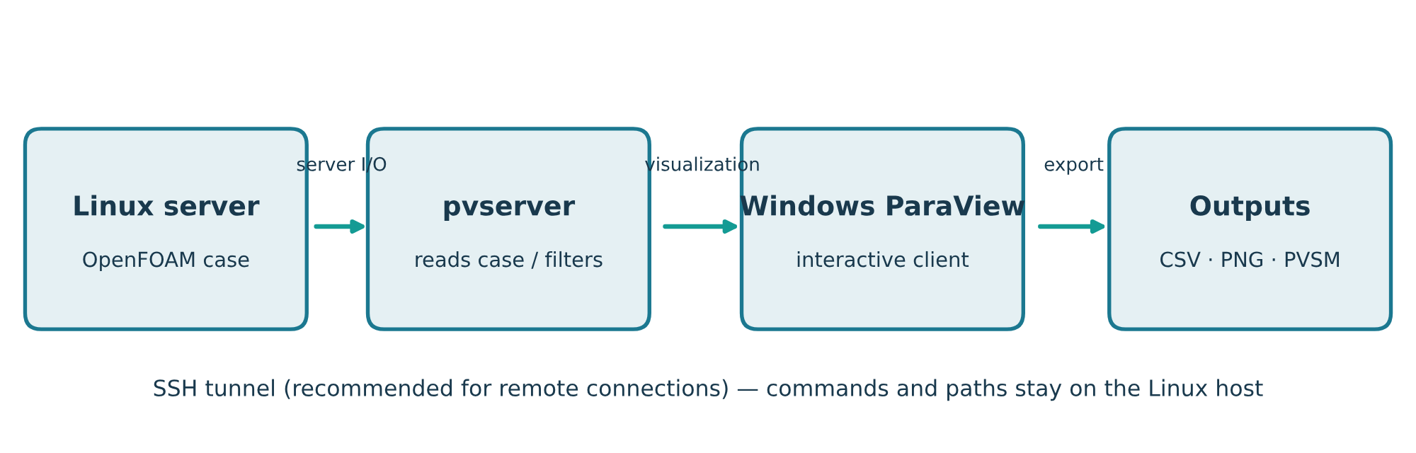
2. Opening a case from Windows through pvserver
2.1 Before connecting
The ParaView client and server must have compatible versions, preferably exactly the same version (5.13.2 in this guide). On Linux, check:
foamVersion
pvserver --version
cd ~/cases/myCase
pwd
ls -d 0 constant system
A placeholder file may be created in the case directory to trigger ParaView’s native OpenFOAM reader:
touch myCase.foamThis empty file is a pointer to the case directory; it is not a results file. The actual reader must exist on the server because that is where file I/O occurs. OpenFOAM’s separately compiled paraFoam/PVFoamReader integration is a different route and may have different version constraints. If no reader works, consider foamToVTK and verify which arrays were exported. For decomposed parallel cases check the native reader’s reconstructed/decomposed case options.
2.2 Example secure connection
Start pvserver on the Linux host in a persistent terminal session:
pvserver --server-port=11111In another Windows PowerShell terminal, start a local SSH tunnel and keep the terminal open:
ssh -N -L 11111:127.0.0.1:11111 USER@SERVERIn Windows ParaView choose File → Connect → Add Server, connection type Client / Server, host localhost, port 11111, then Connect. The SSH tunnel and the Linux server’s network/firewall rules must be correctly configured: do not expose the raw pvserver port directly to the Internet. If local port 11111 is busy, use 11112:127.0.0.1:11111 and connect locally to port 11112.
Once connected, File → Open browses the Linux server’s filesystem, not Windows drive C:. Open myCase.foam, click Apply, and enable the required regions and arrays. If p or U appears to be missing, inspect reader properties, selected timesteps and regions.
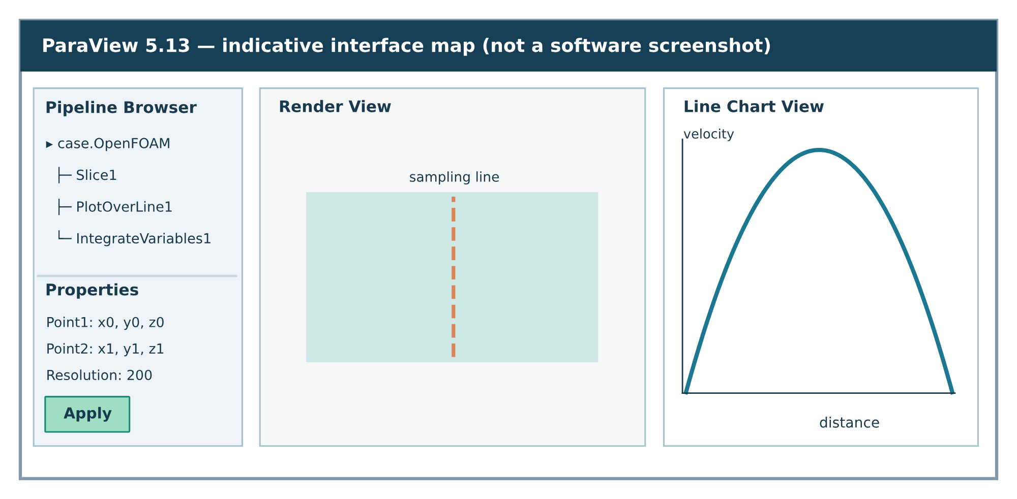
Efficiency rule. Apply filters on the server, export small CSV datasets and retrieve them with FileZilla when needed. Avoid routinely copying complete 3D simulation cases onto Windows.
Deep dive · Restricting pvserver to loopback, as in the first guide
The command pvserver --server-port=11111 listens on every network interface of the server; protection is then left to the firewall. With ParaView 5.13 add --bind-address=127.0.0.1, so the port is reachable only through the SSH tunnel, which delivers traffic to 127.0.0.1:
pvserver --server-port=11111 --bind-address=127.0.0.1The first guide uses this form and also shows a ~/.ssh/config file with LocalForward, which reduces the connection to ssh cfd-paraview. On a shared server each user should have their own port, with the same number in all three places (tunnel, pvserver, ParaView).
Deep dive · OpenFOAM reader options that change the numbers
- Create cell-to-point filtered data (on by default): besides the original cell data it creates interpolated point data with the same name. A filter using point arrays works on interpolated values, not on the ones OpenFOAM computed.
- Mesh Regions:
internalMeshis the fluid volume; patches (patch/inlet,patch/outlet, …) are separate surfaces, useful for integrals over inlet and outlet. - Case Type:
ReconstructedorDecomposed; the latter readsprocessor*/without reconstruction. - Skip Zero Time: hides
0/; turn it off to check initial conditions. - Decompose polyhedra: relevant for meshes with general polyhedra (snappyHexMesh); for blockMesh hexahedral meshes it changes nothing.
3. Understand the underlying arrays first
- Select the case source in the
Pipeline Browserand consultInformation: check bounds, time, cell/point counts and available fields. - Check the actual dimensions in OpenFOAM field files (
0/p,0/Uetc.). A ParaView colour bar usually shows only the field name, not a verified physical unit. - Determine whether fields are Cell Data or Point Data.
Cell Data to Point Datainterpolates cell values; useful for visualization, but not identical to the source discrete values. - Display
Surface With Edgesto inspect the mesh, thenSurfacefor results. Specify consistent colour ranges and record units. - In nominally 2D cases using extruded meshes with
emptyboundaries, distinguish the computational extrusion thickness from the apparatus’s true physical width.
Background — kinematic pressure. Many incompressible OpenFOAM cases store p in m²/s² (kinematic pressure). At constant density rho, a pressure difference in pascals is DeltaP [Pa] = rho [kg/m³] × Deltap [m²/s²]. Check the actual field dimensions in compressible and other model configurations; never multiply every pressure by density unconditionally. Pressure differences are independent of a consistently applied additive pressure reference.
Useful exploratory filters
- Slice: select an origin and a plane normal; this samples an interior section. Areas blocked by solids are not part of the fluid section.
- Clip: removes part of a dataset to reveal the interior; it does not automatically produce the desired measurement section.
- Threshold: isolates cells in a chosen scalar range. Selection semantics depend on point/cell association and inclusion settings.
- Gradient: computes derivatives and, optionally, divergence, vorticity and Q-criterion. Derivatives are especially sensitive to the mesh and any interpolation.
4. Extracting profiles and making graphs
4.1 Plot Over Line
Select the source containing U, usually the case or fluid-region branch. Choose Filters → Data Analysis → Plot Over Line, or find it through the filter search. Define endpoints such as (x0,y0,z0) and (x1,y1,z1), set an initial resolution of about 100–300 samples, then click Apply.
In Line Chart View, select only the desired component (usually U_X, or the X component of U in the reader) or velocity magnitude. Inspect the horizontal axis: label it as distance along the line or an appropriate coordinate rather than assuming the two are interchangeable. Samples outside the fluid domain may be invalid or separated by gaps: do not bridge solids by blind interpolation.
To export values, select the PlotOverLine output, then File → Save Data… and a CSV writer. Check point/cell association and selected output arrays. Column headings vary by reader and ParaView version, so inspect the exported file before downstream calculations.
Deep dive · Sampling pattern and CSV columns
In ParaView 5.13 Plot Over Line has a Sampling Pattern option:
Sample Uniformly: N equally spaced points, interpolated values; the number of points is theResolution.Sample At Cell Boundaries: one sample where the line enters and leaves each cell.Sample At Segment Centers: one sample at the centre of each segment inside a cell; with cell data it returns OpenFOAM’s computed values without interpolation.
In the exported CSV the coordinates appear as Points:0, Points:1, Points:2, vector components as U:0, U:1, U:2, distance along the line as arc_length; the vtkValidPointMask column is 0 for points outside the mesh and must be used to discard them.
4.2 Probe and time dependence
Probe samples the field at a specified location. Verify that the point actually lies in a fluid cell. For changing solutions, explore Plot Selection Over Time or OpenFOAM’s postProcessing/probes files (Guide 2). A Plot Over Line graph at one time is a spatial profile, not a time history.
4.3 Calculator and derived variables
Calculator creates an array from existing fields. For flow aligned with X, select the X component of U from the UI rather than typing an assumed component spelling that could differ across readers. Give the new array a descriptive name such as U_axial. For an incompressible constant-density case with kinematic pressure, a field p_Pa = rho × p can be calculated using the documented numerical value of rho. Do not apply this conversion in the wrong physical model.
Deep dive · The same profile with a pvpython script
Repeated operations (the same profile on several cases or times) are better scripted. ParaView ships pvpython and pvbatch, which run directly on the server without a GUI. The script reads the case, takes the last time, applies Plot Over Line and exports the CSV next to the case:
# profile.py  -  run on the server:  pvbatch profile.py   (or pvpython)
from paraview.simple import *

case = '/home/USER/cases/caseName/caseName.foam'
r = OpenFOAMReader(FileName=case)
r.MeshRegions = ['internalMesh']
r.CellArrays = ['p', 'U']
r.UpdatePipelineInformation()
t = r.TimestepValues[-1]                 # last written time

pol = PlotOverLine(Input=r)
pol.Point1 = [0.08, -0.001, 0.0]         # line end points: adapt them to your domain
pol.Point2 = [0.08,  0.001, 0.0]
pol.Resolution = 200
pol.UpdatePipeline(t)

SaveData('/home/USER/cases/caseName/profile_x080.csv', proxy=pol,
         PointDataArrays=['U', 'p', 'arc_length', 'vtkValidPointMask'])
print('wrote profile_x080.csv at time', t)
A quick way to get a starting script is Tools → Start Trace: ParaView records the GUI operations in Python, and Stop Trace shows the code to save and adapt.
5. Section means, pressure drop and flow rate
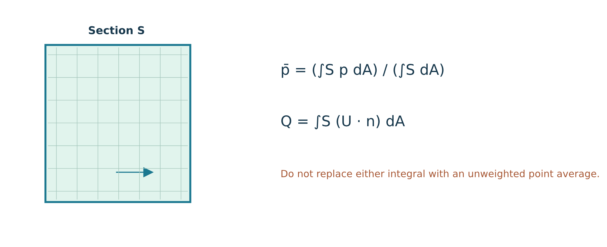
On a fluid cross section S, area-weighted mean pressure and volumetric flow rate are
[ \overline{p}_S = \frac{\int_S p\,dA}{\int_S dA}, \qquad Q_S = \int_S \mathbf{U}\cdot\mathbf{n}\,dA. ]
Integrate Variables produces the integrals, not a ready-made average. For a plane perpendicular to X, integrating the U_x component yields a signed volumetric flow rate according to your chosen +X convention; for arbitrary planes use the component normal to the surface.
Procedure with unambiguous definitions
- Apply
Sliceto the original case using plane normal X atx = x_A. Confirm that the output is the intended fluid cross section, excluding solid blocks and irrelevant boundaries. When a suitable inlet/outlet patch is already present,Extract Blockmay be preferable. - Apply
Integrate Variablesto thisSlice. Inspect the integral of pressure inSpreadsheet View/Information, and obtain the Area when exposed by the filter. If necessary, useCalculatoron the same slice to create a constant arrayone = 1and integrate that as the area. Computep_mean = integral(p)/Area. - Repeat at
x = x_Bwith the same definitions and obtainDelta p = p_mean,A − p_mean,B. Convert to Pa if, and only if,pis kinematic pressure and density is constant. - Use
Calculatoron a section normal to X to obtainU_axial = Ux, then applyIntegrate Variables. The signed result isQ = integral(U_axial)with the +X convention. For a general section computeintegral(U · n)using a consistently oriented normal. - Compare
Qfrom at least two sections. For incompressible steady flow, they should agree within a justified tolerance. With varying density, compare the mass flow ratem_dot = integral(rho U · n)instead.
Important. Integrating |U| is not the normal flow rate unless the velocity happens to be normal everywhere and points in the same direction. Integrating pressure on a wall patch is not the same quantity as the area-mean pressure on a fluid section.
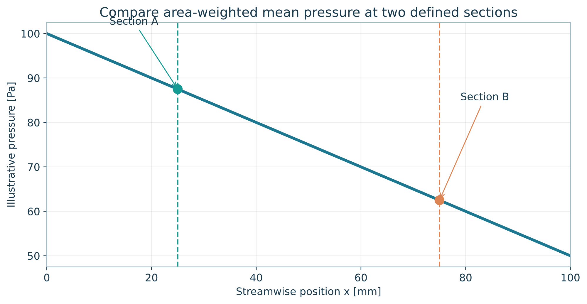
Background — orientation and signs. If boundary patch normals point outward from the fluid volume, inlet flow has a negative signed rate and outlet flow a positive signed rate. Check conservation through the signed sum, not by arbitrarily changing signs to make two numbers look alike.
Deep dive · Integrate Variables: area, cell data and direct averages
- On a surface the filter returns an
Areacolumn; on a lineLength; on a volumeVolume. It is the geometric measure of the integrated domain: compare it with the expected section area as a first check. - It integrates both point and cell data, in two tables (attribute selectable in the
Spreadsheet View). On aSlicecell data are the values of the cut cells, point data are interpolated: on fine meshes they agree, on coarse ones they do not, and the difference indicates the measurement uncertainty. - The Divide Cell Data By Volume option divides cell-data integrals by the domain measure (the area, for a section): it returns the area-weighted average of cell data directly.
An independent cross-check from outside ParaView is the surfaceFieldValue function objects of the second guide: on inlet and outlet both methods must give the same flow rate.
6. Exercise 1 — Laminar channel and Poiseuille profile
Goal. Extract U_x(y) from a fully developed region, compare it with the analytical profile and report a reproducible error measure.
Required case. A straight channel with incompressible laminar flow, no-slip walls and constant section. This guide does not ship a ready-to-use OpenFOAM case. Use a copy of a validated introductory case. The theoretical formula only applies to steady, fully developed planar flow without additional acceleration effects.
Consistent illustrative parameters: full channel height H = 0.002 m, measurement length L = 0.100 m, density rho = 1000 kg/m³, dynamic viscosity mu = 0.001 Pa·s, bulk velocity U_mean = 0.100 m/s; physical width for volumetric flow, if relevant: W = 0.010 m. These give Re_H = rho·U_mean·H/mu = 200 and the ideal planar profile
[ U_x(y)=\frac32 U_{mean}\left[1-\left(\frac{2y}{H}\right)^2\right],\quad -H/2\le y\le H/2. ]
The analytical maximum is U_max = 0.150 m/s, while the predicted fully developed pressure drop is DeltaP = 12 mu L U_mean/H² = 30 Pa (Delta p = 0.030 m²/s² if stored as kinematic pressure). The physical flow rate is Q = U_mean H W = 2.0 × 10⁻⁶ m³/s. These are analytical targets, not CFD measurements.
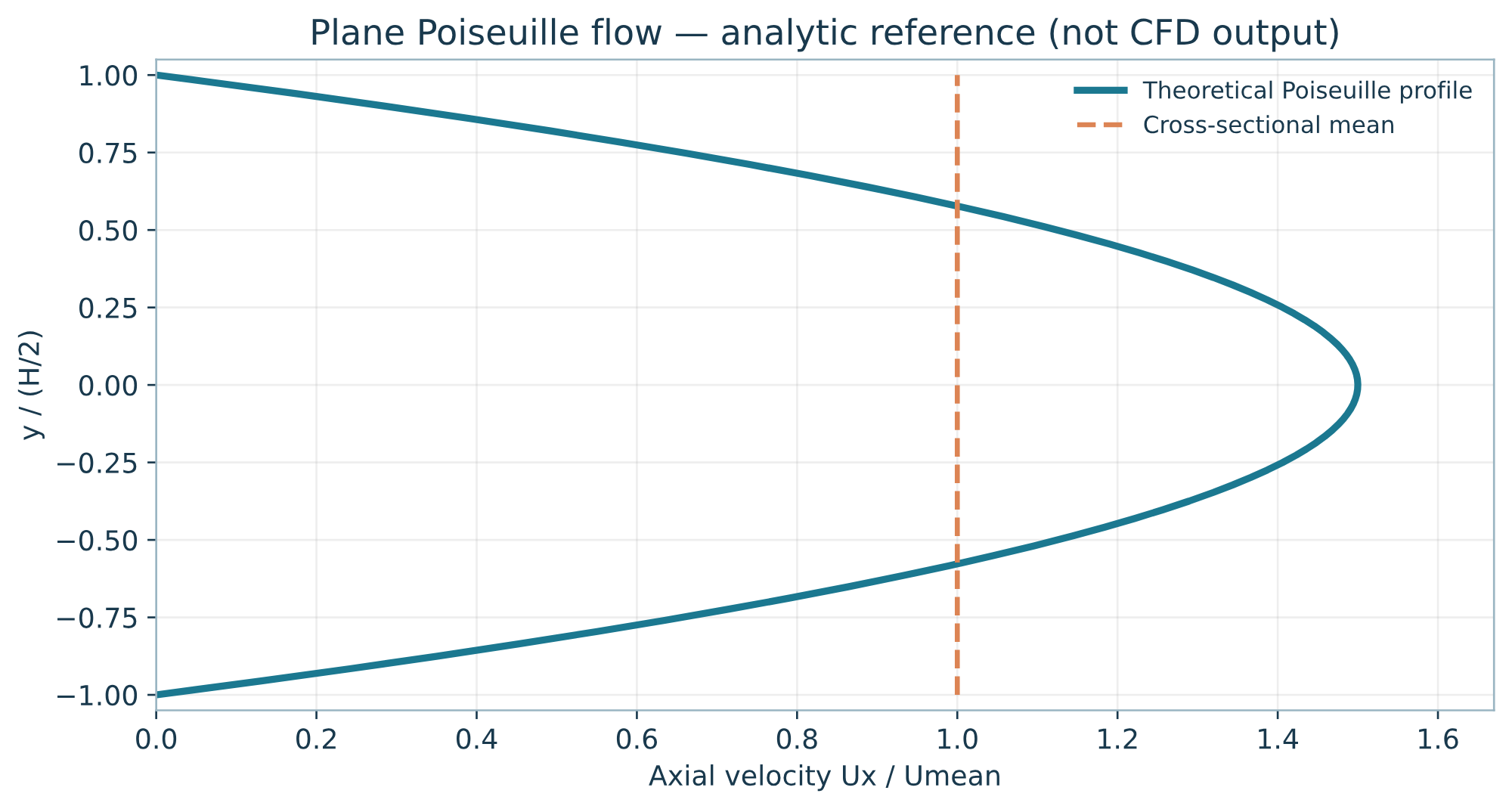
Workflow. Open the converged final step. Apply Plot Over Line along Y in a section well downstream of inlet effects, with endpoints inside the fluid. Export position Y and U_x. In a spreadsheet construct columns for y, U_CFD, U_theory, difference and squared difference. Only compare valid samples at matching physical coordinates and with consistent normalization.
Error, for N paired samples on the same comparison grid:
[ RMSE=\sqrt{\frac1N\sum_{i=1}^{N}(U_{CFD,i}-U_{theory,i})^2},\quad RMSE_{rel}=100\,RMSE/U_{mean}. ]
The relative error is explicitly normalized by U_mean, ensuring a reproducible definition for later mesh comparisons. examples/poiseuille_reference.csv includes an analytic sampled profile for checking the spreadsheet workflow before CFD data are available.
Final checks. Check no-slip at walls, approximately 1.5·U_mean at the centreline, symmetry, negligible profile change between two subsequent sections, and agreement between the flow rate integrated by ParaView and the section-mean estimate. Do not treat the 30 Pa analytical target as an acceptance criterion for an entrance region that is not fully developed.
Deep dive · Computing RMSE in Python from the ParaView CSV
The script uses ParaView’s standard CSV column names, discards points outside the fluid and compares with the Poiseuille formula. yc is the channel axis coordinate: if the mesh runs from 0 to H, set yc = H/2.
# rmse_poiseuille.py  -  python rmse_poiseuille.py profilo_x080.csv
import csv, math, sys

H, Umean = 0.002, 0.100                    # case data
yc = 0.0                                   # y coordinate of the channel axis
rows = list(csv.DictReader(open(sys.argv[1], newline='')))
pts = []
for r in rows:
    if r.get('vtkValidPointMask', '1') in ('0', '0.0'):
        continue                           # point outside the fluid
    y = float(r['Points:1']) - yc
    u = float(r['U:0'])                    # x velocity component
    if abs(y) <= H / 2:
        pts.append((y, u))
err2 = [(u - 1.5 * Umean * (1 - (2 * y / H) ** 2)) ** 2 for y, u in pts]
rmse = math.sqrt(sum(err2) / len(err2))
umax = max(u for _, u in pts)
print(f'N = {len(pts)}  RMSE = {rmse:.4g} m/s  RMSE_rel = {100 * rmse / Umean:.3g} %')
print(f'U_max CFD = {umax:.4g} m/s  (theory {1.5 * Umean:.4g})')
With Sample At Segment Centers (section 4) the points coincide with the centres of the crossed cells and the error measures the numerical solution, not ParaView’s interpolation.
Deep dive · Where the flow is really developed
At the inlet the profile is flat and becomes parabolic along an entrance length. For laminar duct flow a widely used first estimate is L_e ≈ 0.05·Re·D_h, with D_h the hydraulic diameter (for two parallel plates D_h = 2H). With the exercise data Re_Dh = 400 and L_e is of the order of 8 cm: a profile measured a few millimetres from the inlet cannot be compared with Poiseuille.
The practical criterion is the guide’s: two profiles at consecutive sections must coincide. If they do not, the measurement section is still in the development region, or the channel is too short for the chosen Reynolds number.
7. Exercise 2 — Pressure drop through a flow component
Goal. Obtain a reproducible DeltaP measurement and compare multiple flow rates or geometries.
Setup. Place two well-defined planes upstream and downstream, far enough from artificially imposed boundaries to avoid misleading values. Record plane coordinates and areas. Avoid planes crossing solids, no-data regions, and numerically perturbed inflow regions. Whenever possible keep the same measurement definitions in comparisons between geometry variants.
- Create
Slice_inandSlice_outwith documented normals and coordinates. - On each, integrate pressure, measure area and compute the area-weighted mean pressure.
- Verify signed flow rate using
integral(U · n)(or axial component for a properly aligned plane). - Convert the difference to Pa only when the units require it.
- Save
Q,DeltaP,rho,mu,x_A,x_B, time, mesh and case identifier in a table. - Repeat for other flow rates without silently changing measurement-plane definitions. Plot
DeltaP(Q)and indicate departures from a linear relationship.
Illustrative numbers only, not OpenFOAM output: p_mean,A = 0.120 m²/s², p_mean,B = 0.085 m²/s², rho = 998 kg/m³ give DeltaP = 998·(0.120−0.085) = 34.93 Pa. A physical comparison can be invalid even between two numerically converged solvers if the sampling planes do not represent the same measurement.
Background — static pressure and head loss. When inlet and outlet sections have different area or kinetic-energy flux, a static-pressure difference is not necessarily equal to the irreversible energy loss. State which quantity is being reported: static pressure difference, total pressure difference or an appropriately defined loss coefficient.
Deep dive · Total pressure and loss coefficient with Calculator
With kinematic pressure, kinematic total pressure comes from a Calculator on cell data:
p_tot = p + 0.5*mag(U)^2The area-weighted average of p_tot on the two sections gives the total pressure loss Δp_tot; the dimensionless loss coefficient is K = Δp_tot / (½·U_ref²) (kinematic form, no density), with U_ref the mean velocity of a stated section. For more rigour the total pressure average should be flow-weighted (∫ p_tot U·n dA / Q): with strongly non-uniform profiles the two averages differ, and you must state which one you use.
8. Exercise 3 — Wakes and recirculation regions
Suggested case. The official OpenFOAM Foundation 14 tutorial incompressibleFluid/pitzDailySteady, featuring a backward-facing step. Copy it to a personal case directory and run it according to the v14 User Guide; do not modify the installed tutorial. This is a quasi-two-dimensional numerical configuration, not a universally valid model of 3D separation.
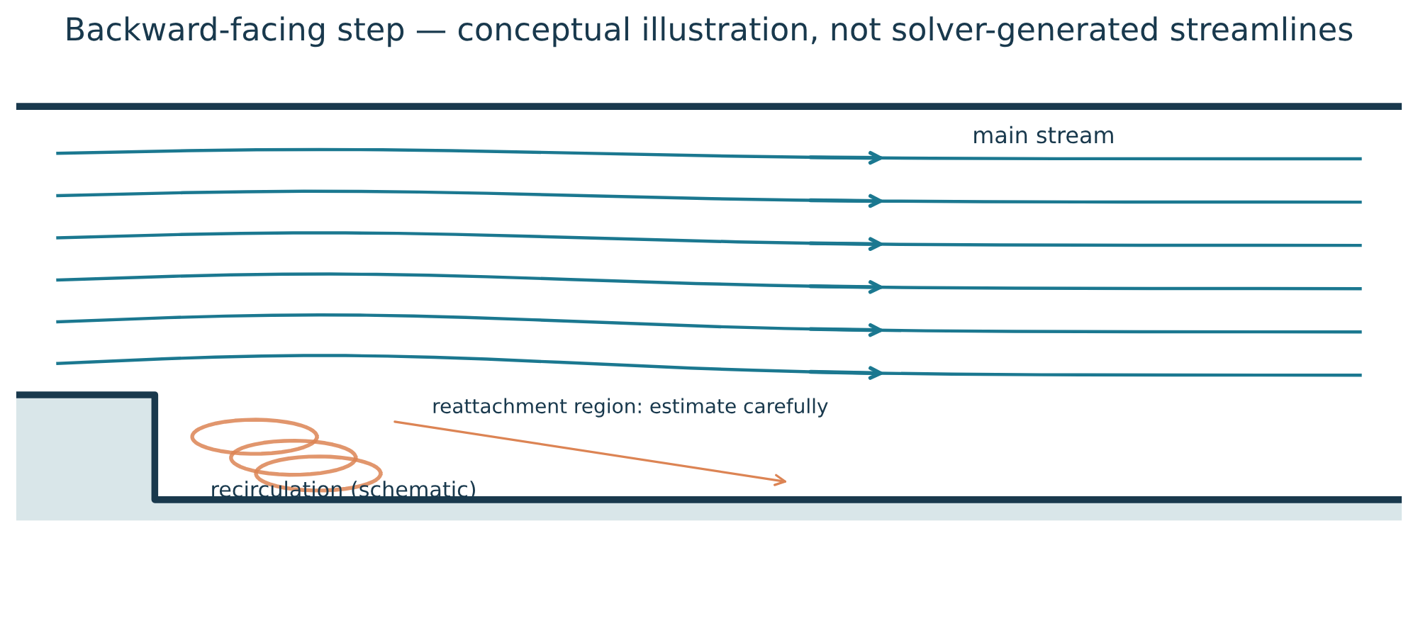
Part A — visual exploration. Display U on an internal slice of the final solution. Apply Stream Tracer, seed inside the fluid near the upstream section and select vector field U. Inspect maximum streamline length and integration direction. Streamlines follow the instantaneous velocity field and are not necessarily particle trajectories in unsteady flows.
Part B — quantitative region selection. For average flow directed along +X, use Calculator to create U_axial, then Threshold to retain cells where U_axial < 0. Make sure the data association matches the intended source field. For an extruded nominally 2D case, volume integration of the selected U_x < 0 region includes the numerical thickness; to measure 2D area, use an appropriate planar slice. Clearly state the measurement’s dimensions and selection rule.
Part C — physical interpretation. Extract U_x(y) profiles at several downstream positions and inspect negative velocity and the shrinking separated region. Reattachment length is not automatically the coordinate where a coloured streamline ends; it needs a declared operational definition, such as the position where sampled wall shear stress crosses zero with appropriate sign. If results are sensitive to mesh refinement, report that dependence rather than presenting a single precise-looking number. Numerical validation is addressed in Guide 4.
Deep dive · Measuring reattachment with wall shear stress
OpenFOAM computes wall shear stress with the wallShearStress function object. On written times it is applied in post-processing, naming the solver module because the momentum transport model and turbulence fields are needed:
foamPostProcess -solver incompressibleFluid -func wallShearStress -latestTimeThe wallShearStress field is written in the latest time directory. In ParaView: reload the case, select in Mesh Regions the lower wall patch downstream of the step, apply Plot Over Line (or Plot Data on the patch) and read where the X component changes sign. Check the sign convention in the attached-flow region far from the step and use the sign change, not the absolute value.
The Q criterion, available in the Gradient filter (Compute QCriterion), highlights vortices in shear regions, but the isosurface threshold is arbitrary: state it alongside the image.
9. Comparing cases, exporting and preserving work
9.1 Meaningful comparisons
Use a measurement table (template included) with one row per case: mesh, boundary conditions, density, viscosity, flow rate, pressure drop, measurement locations and time. Overlay profiles only when coordinates and units agree. When comparing datasets from different meshes, export CSVs and interpolate onto a shared sampling grid with the interpolation procedure stated. Do not subtract rows from two nonaligned files.
9.2 Windows-friendly output
File → Save Data…: select the correct pipeline output before saving CSV. In a client/server session inspect where the destination dialog writes the result; some data exports are performed on the server and can then be retrieved with FileZilla.File → Save Screenshot…: specify resolution, labels and consistent colour bars; scientific figures should identify field, units and colour range.File → Save State…writes a.pvsmpipeline description.File → Load State…restores the pipeline but does not embed CFD datasets; ParaView may request new paths. A state tied to a remote server can need reconnection and dataset path remapping.- Preserve CSV and PVSM outputs with a measurement record. PNG pictures alone are not sufficient for reproducing numerical values.
Suggested organization on Windows:
CFD_analysis/
  01_case_and_conditions.txt
  02_profiles_csv/
  03_sections_and_integrals/
  04_figures_png/
  05_paraview_state/
  06_report/
Excel or LibreOffice Calc can analyse the CSVs; Notepad++ can inspect headers and raw text; FileZilla retrieves outputs from Linux. No IDE is required. There is usually no reason to transfer full volumetric fields just to plot a velocity profile.
Deep dive · States, scripts and reproducibility
- A
.pvsmstate is an XML file: it can be opened in Notepad++ to see paths, filters and parameters, and to fix a server path before reloading. File → Save State…also offers the Python format (.py): the same state becomes a script runnable withpvpythonorpvbatch, useful to redo the analysis on another case by changing one path.- For mesh comparisons, a script like the one in section 6 applied to each mesh’s CSV yields one table row per mesh, with the same points and the same error definition.
10. Frequent problems and practical checks
| Symptom | Likely cause | Action |
|---|---|---|
Windows C: drive missing in Open dialog | pvserver file I/O occurs on Linux | Navigate to a Linux path |
Fields U or p absent | Incorrect reader selection/region/time | Reader Properties, Apply, Information |
| Line profile contains gaps | Line partly outside fluid | Revise endpoints and validity mask |
| Integrated result is implausible | Wrong geometry, array association or units | Verify area and filter input |
| Pressure drop differs by ~1000× | Kinematic pressure treated as Pa | Inspect OpenFOAM field dimensions |
| Signed flow rate changes sign | Normal is reversed | Document +/− convention |
| No streamlines | Seeds in solids or wrong vector field | Relocate seeds, choose U |
| Very slow filters | Too many arrays/regions, very large data | Disable unused arrays; filter server-side |
| PVSM state fails to restore | Dataset paths changed, server disconnected | Reconnect pvserver, relink data |
| Images look similar but profiles differ | Representation masks actual differences | Compare quantitative CSV values |
11. Reproducible measurement checklist
Before publishing or sharing a result, record the following (CSV template supplied):
- Case ID/version, OpenFOAM and ParaView versions, date and original case path.
- Field dimensions, final units, and whether
pis physical or kinematic pressure. - Simulation time/iteration, mesh and relevant boundary conditions.
- Sampling line or plane positions, normals, areas or thicknesses, and selected blocks.
- Filter names and parameters (
Plot Over Line,Calculator,Integrate Variables, etc.). - Measurements and an independent check (at least a flow balance or applicable analytical expectation).
- Deliverable files (CSV, labelled PNG chart, PVSM state) and stated interpretation limits.
Learning outcome. Readers should be able to extract a velocity profile and RMSE, compute volumetric flow rate and pressure drop, distinguish flow recirculation from visualization artifacts, and deliver results another user can independently reconstruct.
Deep dive · A measurement sheet template in CSV
One row per measurement, with these columns, opens in any spreadsheet and keeps data, method and files together:
case_id,time_or_iteration,mesh_cells,field,field_dimension,rho_kg_m3,mu_Pa_s,section_A_x_m,section_B_x_m,area_A_m2,area_B_m2,p_mean_A_field_units,p_mean_B_field_units,deltaP_Pa,Q_A_m3_s,Q_B_m3_s,method_notes,csv_file,pvsm_fileThe field_dimension column (for example kinematic_m2_s2) prevents the most common mistake, applying or forgetting the rho factor.
Official references and figure notes
- ParaView 5.13.2 — Filtering Data — Slice, Plot Over Line, Calculator, Gradient, Integrate Variables.
- ParaView 5.13.2 — Remote and parallel visualization — client/server connections and SSH tunnels.
- ParaView 5.13.2 — Saving Results — exports and PVSM states.
- ParaView 5.13.2 — Targeted: Computational Fluid Dynamics — CFD streamline filters.
- OpenFOAM Foundation v14 — ParaView — OpenFOAM readers and post-processing.
- OpenFOAM Foundation v14 — Backward-facing step —
pitzDailySteadytutorial. - OpenFOAM Foundation v14 — Field format and dimensions — field dimensions and unit conventions.
Figure provenance: all embedded figures were newly drawn for this guide; they are either operational schematics or analytic reference graphs. The GUI map is a reconstruction, not an actual ParaView screenshot. Illustrative plots are not CFD results unless explicitly stated otherwise. Filter descriptions were checked against the official documentation.
Related guides: OpenFOAM on a Linux server, working from Windows, monitoring, troubleshooting and convergence assessment and the Learning OpenFOAM 14 path.