

OpenFOAM: verification, validation and mesh independence
Fourth operating guide on OpenFOAM installed on a Linux server and used from Windows, after those on server and transfers, monitoring and convergence and quantitative analysis with ParaView. This one answers the question that comes next: is the result reliable enough to answer a physical question? Reference: OpenFOAM Foundation 14.
OpenFOAM Foundation 14 · Windows client + Linux server · CFD operations handbook
Purpose. Determine whether a CFD prediction is reliable enough to answer a specific physical question. This handbook provides a repeatable protocol using three related meshes, conservation checks, an analytical benchmark and an indicative estimate of spatial-discretization uncertainty. The numerical values in the GCI exercise are synthetic; they are not OpenFOAM solver results.
Prerequisites. Basic SSH access, FileZilla file transfers and Notepad++ editing (Guide 1); log monitoring and residuals (Guide 2); quantitative measurements using ParaView client/server (Guide 3). Visual Studio Code is neither required nor discussed. Optional background callouts can be skipped by readers with a CFD background.
1. What makes a CFD result trustworthy?
An iteratively converged solution may still be inaccurate. A result may barely change under mesh refinement yet represent the wrong physics. Mass conservation does not guarantee that pressure drop or recirculation has been predicted correctly. Keep four distinct questions in mind:
| Assessment | Question | Minimum evidence |
|---|---|---|
| Iterative convergence | Are the discrete equations solved sufficiently well? | Residuals and stable quantities of interest |
| Spatial verification | Does the output change with mesh refinement? | Three comparable meshes and error estimate |
| Temporal verification | Does the time step influence the answer? | At least three deltaT values for transient runs |
| Physical validation | Does the model reproduce physical reality? | Independent benchmark/measurement and uncertainty |
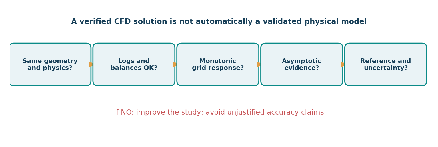
Verification concerns the solution of the selected equations; validation asks whether those equations, assumptions and boundary conditions represent the physical system. checkMesh reporting Mesh OK is not evidence that a physical model has been validated.
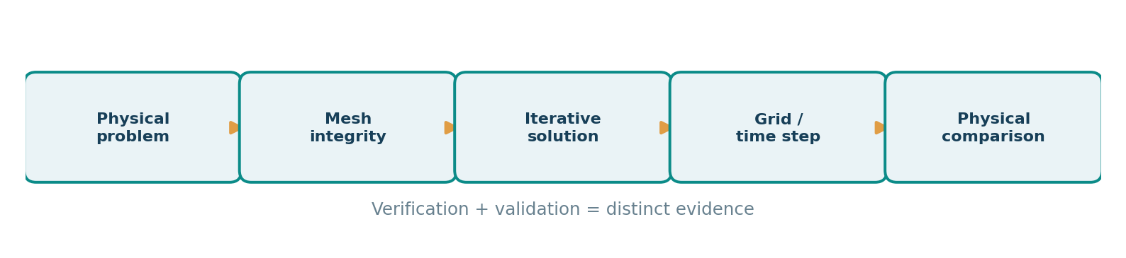
Background — errors and uncertainties. Iterative error arises because an iterative solver stops; discretization error arises from the spatial and temporal approximations; input and experimental uncertainties arise from missing knowledge of conditions or measurements. A grid-convergence statistic does not encompass all these effects.
Deep dive · Code verification and solution verification
The CFD credibility literature (Roache; Oberkampf and Roy; the ASME V&V 20 standard) distinguishes three levels:
- Code verification: does the program solve the mathematical model correctly? It is checked with exact or manufactured solutions, measuring that the error decreases at the formal order of the schemes. It is the developers’ job; the user repeats it on a small scale with a case of known solution, such as Poiseuille.
- Solution verification: how large is the numerical error of this run? Iterative convergence, mesh and time-step studies, GCI. It is the core of this guide.
- Validation: does the model represent reality with the required accuracy? It needs reference data with their own uncertainty.
The order matters: without solution verification you do not know how much of the difference from the experiment is numerical error, and validation becomes a comparison between two numbers of unknown origin.
2. Define the quantity of interest before computing
Choose a quantity of interest (QoI) before running your cases: pressure drop between two fixed planes in Pa, flow rate in m³/s, a velocity component at a specified location, reattachment length in m or a species flow in mol/s. Use the same extraction method across meshes.
| Item | Explicit example |
|---|---|
| Physical system | Two-dimensional fully developed laminar channel |
| Primary QoI | DeltaP = pA - pB across fixed planes |
| Imposed condition | Mass flow or mean velocity, not arbitrary simultaneous values |
| Units | Verify whether p is kinematic pressure or pressure in Pa |
| Target | Fine/medium DeltaP difference < 1% and defensible GCI study |
| Independent reference | Analytical expression, verified benchmark or experimental data |
The 1% target is illustrative, not a universal standard. A safety-related threshold or a local derivative could require a very different tolerance.
Deep dive · Integral and local quantities converge differently
Integral quantities (flow rate, mean pressure drop, force on a wall) average local errors and usually converge quickly and smoothly. Local quantities, and especially derivatives (wall shear stress, gradients, local heat fluxes, the position of a reattachment point), converge more slowly and often non-monotonically, because they depend on the resolution in that specific region and on interpolation.
Practical consequence: a mesh “independent” for ΔP may not be so for wall shear stress. The study must be stated per QoI, not for the mesh in general.
3. Keep the physical model fixed: change the mesh only
A grid study cannot be interpreted if geometry, material properties, viscosity, boundary conditions, turbulence closure or extraction planes are also modified. Build a family of geometrically equivalent meshes, not three different CAD models.
Create new case directories while preserving the original:
# Linux SSH session; adapt case names and paths
cd ~/cases
cp -a reference case_M1_fine
cp -a reference case_M2_medium
cp -a reference case_M3_coarse

# Snapshot key numerical setup files
for c in case_M1_fine case_M2_medium case_M3_coarse; do
  ( cd "$c" && sha256sum system/controlDict system/fvSchemes system/fvSolution ) \
    > "$c.input.sha256"
done
If reference includes old fields and output, prefer a clean template to avoid mixing results. Do not delete old results indiscriminately. On each copied case adjust only the meshing parameters.
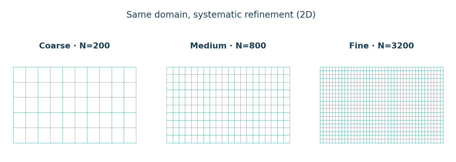
For an extruded 2D mesh with one cell through thickness, a Nx × Ny × Nz sequence such as 20×10×1, 40×20×1, 80×40×1 gives nominal counts of 200, 800 and 3200 with a linear refinement ratio r=2 between adjacent meshes. Cell count grows by four in a 2D uniform refinement.
3.1 Representative size h
For regular refinement in a fixed physical domain, h ~ (V/N)^(1/d) with effective dimensionality d: 2 for genuinely 2D and 3 for 3D. The volume or area must refer to the same physical domain. For anisotropic or nonuniform refinement of unstructured 3D meshes, a single global h based on cell count is merely a rough indicator and does not establish a proper grid refinement ratio.
Deep dive · Generating the mesh family with blockMesh or refineMesh
With blockMesh change only the cell counts in the blocks entry of system/blockMeshDict, doubling the in-plane directions and keeping 1 cell through the thickness:
foamDictionary -entry blocks system/blockMeshDict     # read the current entry
# coarse:  hex (0 1 2 3 4 5 6 7) (20 10 1) simpleGrading (1 1 1)
# medium:  hex (0 1 2 3 4 5 6 7) (40 20 1) simpleGrading (1 1 1)
# fine:    hex (0 1 2 3 4 5 6 7) (80 40 1) simpleGrading (1 1 1)
With simpleGrading other than 1 the last-to-first cell ratio stays the same at every level: doubling the cells halves each cell approximately uniformly and the family remains geometrically similar, even though the ratio between adjacent cells changes. Grading is explained in Part 2: blockMeshDict.
Alternatively refineMesh splits every cell in two along the chosen directions, giving exactly r = 2; in 2D cases a system/refineMeshDict excluding the thickness direction is needed. To shorten runs on fine meshes you can initialise the field from the previous mesh’s solution:
cd ~/cases/case_M2_medium
mapFields ../case_M3_coarse -consistent -sourceTime latestTime
Initialisation only changes the starting point of the iterations: the final solution, if iterative convergence is complete, does not depend on it.
Deep dive · h worked out on the example
For a 2D domain of 0.100 × 0.010 m (area 1.0×10⁻³ m²): with 200 cells h = (1.0×10⁻³/200)^½ = 2.24 mm; with 800 cells 1.12 mm; with 3200 cells 0.559 mm. The ratio between successive values is 2.00, consistent with doubling cells in each direction. For the script the relative h (4, 2, 1) is enough: only the ratio matters.
4. Check each grid, not only the finest
Verify that the OpenFOAM Foundation 14 environment is loaded in the remote shell. For each case:
foamVersion
cd ~/cases/case_M2_medium
blockMesh > log.blockMesh 2>&1   # only if blockMesh generates the mesh
checkMesh -allGeometry -allTopology > log.checkMesh 2>&1

tail -n 35 log.checkMesh
Record cell count, positive volumes, topology checks, non-orthogonality, skewness, aspect ratio where relevant and the distribution of locally refined cells. Mesh OK indicates integrity, not mesh independence. Appropriate quality limits depend on the numerical schemes and the physical problem.
With snappyHexMesh, document wall layers and changes in discretized solid/fluid geometry. Changes in wetted area, opening size or solid volume affect pressure drop in ways that cannot be attributed solely to discretization. With wall turbulence models, document y+ and compatibility with the chosen wall treatment.
Deep dive · Pulling the comparable numbers out of checkMesh
for c in case_M1_fine case_M2_medium case_M3_coarse; do
  echo "== $c"
  grep -E 'cells:|Max non-orthogonality|Max skewness|Max aspect ratio|Mesh OK|\*\*\*' $c/log.checkMesh
done
In a well-built family the cell count scales as rd and quality indicators stay similar or improve with refinement. If the fine mesh has much worse maximum non-orthogonality than the others, the family is not consistent: the study would compare different mesh qualities as well as different sizes.
5. Run three comparable cases and keep an audit trail
The following is a generic example for an already configured case, not a universal command for arbitrary folders:
cd ~/cases/case_M1_fine
# Foundation 14: the solver module may be set in system/controlDict.
# Confirm solver module, initial conditions and models before execution.
foamRun > log.foamRun 2>&1

grep -E 'Time =|ExecutionTime|Solving for|continuity errors' log.foamRun | tail -n 30
For long runs, use tmux as described in Guide 1 and keep the process alive. Repeat the same protocol for each grid. Allrun scripts can trigger multiple operations: inspect with less Allrun before starting; an arbitrary Allrun is not necessarily equivalent to foamRun.
Record computer hardware, foamVersion, source revision, fluid physics, fvSchemes and fvSolution configuration and solver tolerances. For steady cases use a converged final state; for transient problems compare identical physical time or the same statistical time window, not identical iteration numbers.
5.1 Make iterative noise smaller than mesh effects
Before claiming that a change is mesh-induced, verify the QoI is stable under more solver iterations. If additional iterations change DeltaP by 0.8% while two grids differ by 0.5%, the refinement study is not interpretable. Keep a QoI-versus-iteration trace as well as residual plots.
Deep dive · How small the iterative error must be
A recurring practical rule in the verification literature (for example Roy, Oberkampf and the NASA tutorial on iterative convergence) is that the iterative error on the QoI should be at least an order of magnitude smaller than the discretisation error being estimated. With the differences above: if the fine and medium meshes differ by 0.5%, the fine-mesh QoI must be stable to about 0.05%.
A concrete way to estimate it: take ΔP over the last N steps and compute its relative variation and slope, as the monitoring script of guide 2 does. If residualControl tolerances stop the run before this level, tighten them.
6. Use identical measurement definitions across grids
Apply the same ParaView filters (Guide 3) or OpenFOAM function objects. For pressure drop use two fixed physical planes, identical area-weighted pressure averages, the same time definition and consistent units.
For constant-density incompressible flow, if p has dimensions [0 2 -2 0 0 0 0], it is kinematic pressure: DeltaP[Pa] = rho[kg/m3] × Deltap[m2/s2]. When p is already in Pa, do not multiply by rho.
A probe along a line is not an area integral. In a porous or obstructed duct, compare the same physical plane even when the fluid subset intersected by the plane differs. If geometrical reconstructions differ, that is an additional source of variability and must be separately reported.
6.1 Mass balance
For a steady incompressible fluid with impermeable walls, the sum of fluxes oriented outwards from the computational domain should be near zero. For multiple boundaries sum all signed flows and define, for example:
epsilon_m = abs(sum(signed_Q)) / max(sum(abs(inlet_Q)), nonzero_threshold)
Declare the threshold that prevents a zero denominator. For compressible flow use mass fluxes and account for accumulation if transient; the instantaneous net boundary flux need not vanish in a transient problem. Check surface normal directions before summation.
Deep dive · Measuring flow rates and Δp with function objects
The most repeatable way to measure the same quantities on three meshes is to let OpenFOAM do it during the run: the surfaceFieldValue function objects on inlet and outlet (area-weighted averages of p and sums of phi) are described in guide 2, with a script computing ΔP, ε_Q and stability over the final window. Copying the same system/functions into the three cases makes the measurement definition identical by construction.
For internal sections not coinciding with patches, the ParaView procedure of guide 3 (Slice, Integrate Variables) should be saved as a state or script and reapplied unchanged.
7. Verification benchmark: fully developed Poiseuille flow
For fully developed Newtonian laminar flow between two stationary parallel plates separated by H, the analytical expressions are:
u(y) = 6 * Umean * (y/H) * (1 - y/H)
DeltaP = 12 * mu * L * Umean / H^2
With mu=0.001 Pa·s, H=0.010 m, L=0.100 m and Umean=0.020 m/s, the analytical pressure drop is 0.240 Pa. Evaluate the velocity and pressure difference in a region in which the fully developed assumption holds. A uniform inlet in a short duct creates an entrance region and may legitimately differ from this formula. Do not extend it uncritically to turbulent flow or finite-width 3D ducts.
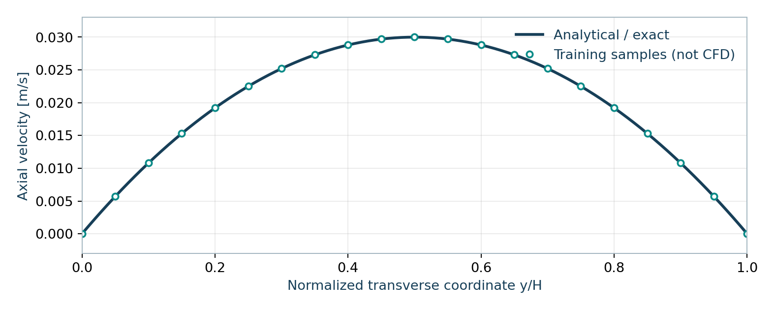
Exercise A. Export at least 21 values of streamwise U_x on a cross-section, compare to the parabola at corresponding y/H, calculate RMSE, peak error and pressure-drop error; also check mass balance. The supplied CSV tables are analytical exercises, not CFD output.
Background — RMSE. RMSE = sqrt(mean((u_CFD - u_theory)^2)). It depends on sampling locations and weights, so specify the positions, interpolation method and sample count. A small profile RMSE does not establish accuracy of every other QoI.
Deep dive · Two ways of writing the same profile
This guide measures y from the lower wall (0 ≤ y ≤ H); guide 3 measures it from the axis (−H/2 ≤ y′ ≤ H/2). With y = y′ + H/2 the two forms coincide:
6 U (y/H)(1 − y/H) = 6 U (½ + y′/H)(½ − y′/H) = 6 U (¼ − y′²/H²) = 3/2 U [1 − (2y′/H)²]
When comparing ParaView CSVs, check where the mesh puts the zero of the transverse coordinate: an H/2 offset shifts the whole parabola and produces a huge RMSE that has nothing to do with the numerical solution.
For an order-of-magnitude check of the exercise: Re = ρ U_mean D_h / μ with D_h = 2H is 400 with ρ = 1000 kg/m³, and the estimate L_e ≈ 0.05 Re D_h gives about 0.4 m: with these data the 0.100 m stretch is developed only if the inlet already imposes the parabolic profile, or if the channel is preceded by a sufficient upstream length.
8. Three-grid study: observed order, Richardson and GCI
Let f1, f2 and f3 be the same QoI on the fine, medium and coarse grids, with h1<h2<h3. Assume a constant linear refinement ratio r=h2/h1=h3/h2>1. Under monotonic, approximately asymptotic convergence, the observed order is:
p = ln(abs((f3-f2)/(f2-f1))) / ln(r)
The Richardson extrapolation based on fine/medium and the fine-grid GCI are:
f_ext = f1 + (f1-f2)/(r^p-1)
GCI_12 = Fs * abs((f2-f1)/f1) / (r^p-1) * 100 [%]
GCI_23 = Fs * abs((f3-f2)/f2) / (r^p-1) * 100 [%]
For three or more grids in the asymptotic region, Fs=1.25 is commonly used. This is not a universal statistical coverage guarantee. A useful asymptotic consistency check is that GCI_23 / (r^p * GCI_12) should be near unity, allowing for the use of f1 and f2 in the respective relative-error denominators. Observed order can differ from the nominal numerical scheme order and is not reliable outside the asymptotic range.
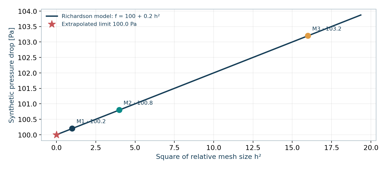
| Grid | 2D cells | Relative h | Synthetic DeltaP [Pa] |
|---|---|---|---|
| M3 coarse | 200 | 4 | 103.2 |
| M2 medium | 800 | 2 | 100.8 |
| M1 fine | 3200 | 1 | 100.2 |
The results are r=2, p=2, f_ext=100.0 Pa, GCI_12≈0.2495%, GCI_23≈0.9921% and a consistency ratio of approximately 0.994. This example was deliberately constructed to show asymptotic convergence. The extrapolated number is not an experimental measurement and does not validate the physics.
Deep dive · The calculation step by step
- Differences:
f2 − f1 = 0.6,f3 − f2 = 2.4; same sign, so monotonic convergence. - Ratio:
2.4/0.6 = 4;p = ln 4 / ln 2 = 2, equal to the formal order of a second-order scheme. r^p − 1 = 3;f_ext = 100.2 + (100.2 − 100.8)/3 = 100.0.GCI_12 = 1.25 × (0.6/100.2) / 3 × 100 = 0.2495%;GCI_23 = 1.25 × (2.4/100.8) / 3 × 100 = 0.9921%.- Check:
0.9921 / (4 × 0.2495) = 0.994.
The same formulas in a spreadsheet, with f1, f2, f3 in B2:B4 and r in B5:
p      =LN(ABS((B4-B3)/(B3-B2)))/LN(B5)
f_ext  =B2+(B2-B3)/(B5^p-1)
GCI12  =1.25*ABS((B3-B2)/B2)/(B5^p-1)*100
GCI23  =1.25*ABS((B4-B3)/B3)/(B5^p-1)*100
check  =GCI23/(B5^p*GCI12)
The safety factor Fs proposed by Roache is 3 for two-grid studies and 1.25 with three or more grids and a verified observed order: the smaller value is the “reward” for having demonstrated the asymptotic range.
8.1 When the straightforward GCI calculation is inappropriate
- The QoI oscillates with refinement:
f3-f2andf2-f1have opposite signs. f2≈f1and iterative noise or round-off dominate the differences.- Adjacent refinement ratios differ; more general equations and a defensible h definition are required.
- Geometry, wall-layer strategy,
y+, models or boundary conditions vary between grids. - The QoI crosses discontinuities, changes flow regime or is unusually sensitive to spatial interpolation.
The packaged gci_three_grids.py deliberately handles only constant-ratio, monotonic three-grid data. Otherwise it exits with a clear diagnostic rather than manufacturing a spurious precision estimate.
Deep dive · Non-uniform ratios and oscillatory convergence
With different ratios r21 = h2/h1 and r32 = h3/h2, the procedure by Celik and co-authors (Journal of Fluids Engineering, 2008) obtains p by iterating:
p = | ln|ε32/ε21| + q(p) | / ln r21, q(p) = ln[ (r21p − s) / (r32p − s) ], s = sign(ε32/ε21)
with ε21 = f2 − f1 and ε32 = f3 − f2. With r21 = r32 the q term vanishes and the guide’s formula is recovered. This is one reason why a constant-ratio family simplifies everything else.
With oscillatory convergence (s < 0) there is no meaningful observed order. A common conservative practice is to state the oscillation amplitude across the three meshes (maximum minus minimum) as the discretisation uncertainty, possibly adding a fourth mesh to see whether the asymptotic range is reached.
Deep dive · The gci_three_grids.py script
Complete script, Python standard library only (3.9 or later). Input: a CSV with columns mesh,cells,h,qoi and rows fine, medium, coarse. It writes results_gci.txt next to the input file.
#!/usr/bin/env python3
"""Guide 04: deliberately conservative equal-ratio, monotonic 3-grid GCI.

Usage: python gci_three_grids.py results_three_grids.csv
Input columns: mesh,cells,h,qoi ; h must be a characteristic size for
geometrically equivalent meshes. The 'mesh' labels must include fine,
medium,coarse (case-insensitive); 'cells' is recorded, not used to infer h.
Generates results_gci.txt next to input. Standard library only, Python >=3.9.
GPL-3.0-or-later example, 2026.
"""
from __future__ import annotations
import csv, math, sys
from pathlib import Path


def calculate(rows):
    required = {"fine", "medium", "coarse"}
    if set(rows) != required:
        raise ValueError("CSV must contain exactly fine, medium, coarse labels")
    x = [rows[key] for key in ("fine", "medium", "coarse")]
    for row in x:
        if row['cells'] <= 0 or row['h'] <= 0:
            raise ValueError("cells and h must be positive")
        if not all(math.isfinite(row[z]) for z in ('cells', 'h', 'qoi')):
            raise ValueError("All numerical values must be finite")
    (f1, f2, f3) = (p['qoi'] for p in x)
    (h1, h2, h3) = (p['h'] for p in x)
    if not h1 < h2 < h3:
        raise ValueError("Must have h(fine) < h(medium) < h(coarse)")
    r12, r23 = h2/h1, h3/h2
    if not math.isclose(r12, r23, rel_tol=0.002, abs_tol=0):
        raise ValueError("Unequal refinement ratios: this simple GCI model does not apply")
    r = (r12*r23)**0.5
    d21, d32 = f2-f1, f3-f2
    if d21 == 0 or d32 == 0:
        raise ValueError("Zero QoI difference: observed order is indeterminate")
    if d21*d32 <= 0:
        raise ValueError("Oscillatory or non-monotonic convergence: no simple GCI")
    if f1 == 0 or f2 == 0:
        raise ValueError("Zero QoI denominator: relative GCI is undefined")
    ratio = abs(d32/d21)
    if ratio <= 1:
        raise ValueError("No positive observed order: no defensible extrapolation")
    p = math.log(ratio)/math.log(r)
    denom = r**p - 1.0
    if not (0 < p < 10) or denom <= 0 or not math.isfinite(denom):
        raise ValueError("Observed order implausible / non-finite; inspect data")
    fext = f1 + (f1-f2)/denom
    fs = 1.25
    gci12 = fs * abs((f2-f1)/f1) / denom * 100
    gci23 = fs * abs((f3-f2)/f2) / denom * 100
    asym = gci23/(r**p*gci12)
    return dict(r=r,p=p,fext=fext,gci12=gci12,gci23=gci23,asym=asym,fs=fs,
                f1=f1,f2=f2,f3=f3, h1=h1,h2=h2,h3=h3)


def read_csv(path):
    out={}
    with path.open(newline='',encoding='utf-8-sig') as f:
        reader=csv.DictReader(f)
        cols=set(reader.fieldnames or ())
        if not {'mesh','cells','h','qoi'} <= cols:
            raise ValueError("Required CSV columns: mesh,cells,h,qoi")
        for row in reader:
            label=row['mesh'].strip().lower()
            if label in out:
                raise ValueError(f"Duplicate mesh label: {label}")
            out[label]={'cells':float(row['cells']), 'h':float(row['h']), 'qoi':float(row['qoi'])}
    return out


def report(a, path):
    return f'''OpenFOAM Guide 04 -- 3-grid GCI (training utility)
Input: {path.name}
Assumptions: identical geometry/physics/measurement, uniform refinement,
             monotonic asymptotic convergence, negligible iterative noise.
Fine/medium/coarse QoI: {a['f1']:.10g} / {a['f2']:.10g} / {a['f3']:.10g}
Characteristic sizes h: {a['h1']:.10g} / {a['h2']:.10g} / {a['h3']:.10g}
Refinement ratio r:          {a['r']:.8f}
Observed order p:            {a['p']:.8f}
Richardson estimate f(h=0): {a['fext']:.10f} [input QoI unit]
Fine-grid GCI12:             {a['gci12']:.6f} %
Medium-grid GCI23:           {a['gci23']:.6f} %
Asymptotic indicator:        {a['asym']:.6f} (near 1 expected)
Safety factor Fs:            {a['fs']:.2f}

CAUTION: GCI is not a total uncertainty budget, does not validate physics,
and is not a confidence interval. Inspect logs and all assumptions.
'''


def main(argv):
    if len(argv)!=2:
        print(__doc__,file=sys.stderr)
        return 2
    path=Path(argv[1])
    try:
        a=calculate(read_csv(path))
        text=report(a,path)
        out=path.with_name('results_gci.txt')
        out.write_text(text,encoding='utf-8')
        print(text)
        print(f'Written: {out}')
        return 0
    except (ValueError, OSError, KeyError, OverflowError) as ex:
        print(f'GCI NOT COMPUTED: {ex}',file=sys.stderr)
        return 1

if __name__=='__main__':
    sys.exit(main(sys.argv))
The test file results_three_grids.csv contains the data of the table above; the expected output is:
Refinement ratio r:          2.00000000
Observed order p:            2.00000000
Richardson estimate f(h=0): 100.0000000000 [input QoI unit]
Fine-grid GCI12:             0.249501 %
Medium-grid GCI23:           0.992063 %
Asymptotic indicator:        0.994048 (near 1 expected)
Safety factor Fs:            1.25
9. Temporal sensitivity: the time step is not the mesh
A spatially converged transient solution may still be wrong because of its time step. With fixed grid and physics, repeat simulations at deltaT, deltaT/2 and deltaT/4, comparing the same QoI at identical physical times after the same startup transient. For periodic signals compare frequency, amplitude, phase and statistics over the same physical window.
Courant number (Co) alone does not establish accuracy. A simulation can be stable at low Courant number and still be overly dissipative. Refining the mesh without addressing the temporal error may hide expected spatial convergence behavior.
Deep dive · Setting up the time-step study in OpenFOAM
- With a fixed step (
adjustTimeStep no) change onlydeltaTincontrolDictand keepwriteControl adjustableRunTimeorrunTime, so written times coincide across the three cases. - With an adaptive step the parameter to halve is
maxCo: the actual step varies in time and the ratio between steps is not exactly 2; read it from the log. - With PIMPLE also fix
nOuterCorrectorsand theFinaltolerances: each step must be iteratively converged, otherwise the study measures the splitting error rather than the temporal one. - The same observed-order and GCI formulas apply with Δt in place of h, provided the compared signal is the same physical instant or the same statistic.
Time-control entries are explained in Part 4: controlDict, PIMPLE algorithms in Part 6.
10. Physics checks and sensitivity to assumptions
Before comparing CFD with the laboratory, perform three distinct assessments:
- Conservation: mass, and when relevant energy and species, including all boundary contributions, source terms and transient accumulation.
- Input sensitivity: vary one realistic uncertain property (e.g. viscosity or inlet flow) at fixed mesh and model; record the QoI response.
- Independent comparison: use an analytical solution, verified reference benchmark or experiment with declared measurement conditions and uncertainties.
If experiment yields DeltaP_exp = 101.0 ± 2.0 Pa (invented illustration) and extrapolated CFD gives 100.0 Pa, numerical proximity is not enough to claim validation. The meaning of ±2.0 and possible model, geometry, input and numerical errors all matter. Do not combine unrelated uncertainty terms in quadrature without an explicit statistical justification and an assessment of correlations.
Deep dive · The comparison in the ASME V&V 20 standard
The ASME V&V 20 standard (verification and validation in fluid dynamics and heat transfer) formalises the comparison as: comparison error E = S − D, the difference between simulation and data; validation uncertainty u_val, which combines numerical uncertainty, simulation-input uncertainty and experimental uncertainty. The quadrature combination u_val = √(u_num² + u_input² + u_D²) assumes the three contributions are independent: exactly the condition the guide asks you to check before using it.
If |E| is of the same order as u_val, model error cannot be distinguished from the “noise” of the uncertainties; if |E| is much larger, there is a model error of about E. In the fictitious example E = −1.0 Pa: without knowing u_val nothing more can be said.
10.1 Geometries reconstructed from images
For geometries obtained from SEM micrographs, photographs, scans or digitized contours, quantify geometric assumptions separately: thickness, curvature, openings and edge location. Increasing mesh density cannot restore missing true geometry. Running plausible alternative geometries is a geometry-sensitivity study, not a grid-convergence study.
11. Worked laboratory: a repeatable protocol
Exercise B — spatial verification. Start from a functioning 2D channel case; build three grids of the same domain; run all cases in OpenFOAM; confirm residual and conservation behavior; extract DeltaP using the same fixed planes; save results_three_grids.csv for analysis on Windows.
The included sample holds synthetic data:
mesh,cells,h,qoi
fine,3200,1.0,100.2
medium,800,2.0,100.8
coarse,200,4.0,103.2
In Windows PowerShell, with optional local Python:
py -3 gci_three_grids.py results_three_grids.csvThe analyzer refuses nonfinite convergence order, unequal ratios or nonmonotonic data. It does not replace critical review of your logs and assumptions. Alternatively, calculate the formulas by hand or in a spreadsheet and document all numerical precision and intermediate steps.
Exercise C — input sensitivity. On an already converged fine mesh change a single physically uncertain input by +5% and -5%, leaving everything else unchanged, and measure the response of DeltaP. Identify this as input sensitivity, never spatial-discretization error.
Deep dive · What to expect in exercise C for a laminar channel
For Poiseuille flow ΔP = 12 μ L U / H² is linear in μ and U: ±5% viscosity or mean velocity gives ±5% ΔP; ±5% of H gives about ∓10%, because ΔP depends on 1/H² (at fixed mean velocity). If the simulation returns sensitivities very different from these, the measured QoI includes other effects (development region, misplaced measurement sections) to understand before going on.
The normalised sensitivity coefficient S = (ΔQoI/QoI)/(Δx/x) sums up the response in one number: 1 for μ and U, about −2 for H here.
12. Organize evidence between Linux and Windows
Keep authoritative cases on the server and use FileZilla to copy only what is needed for review and publication:
CFD_Study_04/
  case_M1_fine/             # server: live cases + logs
  case_M2_medium/
  case_M3_coarse/
  review_windows/
    results_three_grids.csv
    results_gci.txt
    log.checkMesh_M1.txt
    log.foamRun_M1.txt
    figures/
    verification_report.md
Use SFTP to download logs and tables, noting their source directory and transfer date. Notepad++ can inspect and compare dictionaries without changing published copies; ParaView states (.pvsm) should be saved alongside notes about server-side paths, which may be absolute and machine-specific. Record relevant input hashes and program versions.
Deep dive · The verification and validation record
Bilingual template to fill in for every study (Markdown, opens in Notepad++):
# CFD Verification and Validation Record / Scheda di verifica e validazione

## Identification / Identificazione
- Date / Data:
- Operator / Operatore:
- OpenFOAM edition + version / Edizione e versione:
- Case path(s) on Linux server / Percorsi dei casi Linux:
- Windows review directory / Cartella di revisione Windows:
- Input revision or hash / Revisione o hash degli input:

## Physical problem / Problema fisico
- Geometry definition and source / Geometria e origine:
- Boundary and initial conditions / Condizioni al contorno e iniziali:
- Models, properties, units / Modelli, proprietà, unità:
- QoI(s) and measurement protocol / QoI e procedura di misura:
- Acceptance threshold and reason / Soglia accettazione e motivazione:

## Mesh family / Famiglia di mesh
| Grid | Cells | h | r | Worst relevant quality indicator | QoI |
|---|---:|---:|---:|---|---:|
| Fine | | | | | |
| Medium | | | | | |
| Coarse | | | | | |

## Iterative and conservation checks / Convergenza iterativa e bilanci
- Residual and QoI trends / Residui e trend delle QoI:
- Mass imbalance definition + value / Definizione e valore sbilancio massa:
- Time-step verification (if transient) / Studio deltaT (se transitorio):

## Mesh result / Esito di raffinamento
- Observed p / Ordine osservato:
- Richardson extrapolation / Estrapolazione:
- Fine-grid GCI [%]:
- Asymptotic consistency indicator / Indicatore asintotico:
- Non-monotonic / non-asymptotic issues / Eventuali problemi:

## Physical comparisons / Confronti fisici
- Benchmark or experiment and uncertainty / Benchmark o esperimento e incertezza:
- Input and geometry sensitivities / Sensibilità di input e geometria:
- Limitations / Limiti di validità:

## Conclusions / Conclusioni
- Suitability for intended use / Adeguatezza per lo scopo:
- Recommended additional work / Ulteriori verifiche necessarie:
13. Acceptance checklist and responsible conclusions
| Question | Evidence to retain | Status |
|---|---|---|
| Are the three grids geometrically equivalent? | dimensions, fluid volume and generation settings | □ |
| Is mesh quality documented? | three checkMesh outputs and near-wall information | □ |
| Are all three solutions iteratively converged? | logs, residuals and QoI histories | □ |
| Are measurement definitions identical? | planes, averaging, time, units | □ |
| Is conservation error acceptable? | signed flows and normalized imbalance | □ |
| Is grid convergence monotonic and asymptotic? | h–QoI table, observed p, GCI and caveats | □ |
| Is transient resolution sufficient? | deltaT refinement if relevant | □ |
| Is experimental uncertainty characterized? | source, test protocol, interval meaning | □ |
| Does the report state limitations? | geometry, physics, boundaries and numerical assumptions | □ |
Example of a defensible statement. “For the stated domain and boundary conditions, the fine-grid pressure-drop GCI estimate is 0.25%, conditional on uniform refinement and asymptotic convergence. This figure does not include uncertainty in geometry, boundary conditions or the physical model.”
14. Official and methodological references
- OpenFOAM Foundation 14, User Guide: https://doc.cfd.direct/openfoam/user-guide/
- OpenFOAM Foundation 14, Applications and libraries / foamRun: https://doc.cfd.direct/openfoam/user-guide-v14/applications
- OpenFOAM Foundation 14, Post-processing functionality: https://doc.cfd.direct/openfoam/user-guide-v14/post-processing-functionality
- OpenFOAM 14, mesh-check source: https://github.com/OpenFOAM/OpenFOAM-14/blob/master/src/functionObjects/utilities/checkMesh/checkMesh.H
- NASA Glenn / NPARC, Examining Spatial (Grid) Convergence: https://www.grc.nasa.gov/www/wind/valid/tutorial/spatconv.html
- NASA Glenn / NPARC, Examining Iterative Convergence: https://www.grc.nasa.gov/WWW/wind/valid/tutorial/iterconv.html
- NASA Glenn / NPARC, Verification and Validation Tutorial: https://www.grc.nasa.gov/www/wind/valid/tutorial/tutorial.html
- NASA Glenn / NPARC, Examining Temporal Convergence: https://www.grc.nasa.gov/www/wind/valid/tutorial/tempconv.html
- NASA, D. P. Lockard (2010), In search of grid converged solutions: https://ntrs.nasa.gov/api/citations/20100027422/downloads/20100027422.pdf
Scope and limitations. The package includes synthetic training datasets and original explanatory figures. The OpenFOAM instructions are written for adapting existing correctly configured cases. GCI is conditional on its modeling assumptions, not a probability of correctness or experimental validation certificate.
Related guides: Linux server from Windows, monitoring and convergence, ParaView for quantitative analysis and the Learning OpenFOAM 14 path, in particular case 02: mesh convergence study.