

Lesson 11 – Numerical Differentiation and Integration with GNU Octave and GX-TXT
A scientific curve can answer different questions: what is the value of a quantity at a given instant, how quickly does it change, and how much accumulates over time? The first lessons of this course taught us how to create, read, analyse and visualize Datasets with GNU Octave and GX-TXT. We now address the last two questions through numerical differentiation and integration.
We will work with a concentration curve describing first-order kinetics: a synthetic, noise-free experiment that lets us compare every numerical result against a known analytical solution. All scientific computations will be requested through the GX-TXT public APIs, while Octave remains the language in which we organize data, check errors and write scripts.
1. What is new compared with the previous ten lessons?
The course is progressive: understanding this lesson does not require starting again with variables or operators. We do, however, need to distinguish the concepts we already know from the new mathematical operations.
| Topic | Where we encountered it | New concept in Lesson 11 |
|---|---|---|
Variables, vectors, linspace, exp, element-wise operations | Lessons 01–03 and 07 | Using them to build a nonuniform time grid and a verifiable analytical model |
| Loops, conditions, functions and numerical methods | Lesson 04: Euler’s method | Rather than solving a differential equation, estimating derivatives and integrals of sampled data |
| Dataset IDs, Variable IDs and canonical reading | Lessons 05–06 | Checking whether the X axis is suitable for differentiation |
| Atomic publication, units and metadata | Lesson 07 | Assigning physical meaning and dimensions to newly derived results |
| Plot Dataset and debugger | Lesson 08 | Diagnosing a mathematical error raised by the numerical API itself |
| Cumulative mean, empirical distribution and statistics | Lesson 09 | Distinguishing a cumulative statistic from a cumulative integral |
| Regression slope, interpolation and residuals | Lesson 10 | Distinguishing global slope, local derivative and discretization error |
NUMERIC_API_v1 | Already used in earlier lessons | Introducing differentiate, integrate and cumulativeIntegrate |
The fundamental distinction
In Lesson 04 we approximated how a system evolves starting from its differential law. Here, instead, we start from a known sequence of values and want to determine rates of change and accumulated quantities. Both problems involve numerical techniques, but they are not interchangeable.
2. The experiment: first-order kinetic decay
Consider a hypothetical substance whose concentration decreases at a rate proportional to its concentration:
\[\frac{dC(t)}{dt}=-kC(t)\]
The analytical solution of the equation is:
\[C(t)=C_0 e^{-kt}\]
We choose an initial concentration of 4 mmol/L, a rate constant of 0.055 s⁻¹, and an observation interval from 0 to 60 seconds. These examples represent ideal synthetic data: they must not be confused with laboratory measurements or an experimental determination of a kinetic rate constant.
2.1 Why use a nonuniform time grid?
In Lesson 07 we generated sinusoids sampled at constant intervals. In this exercise, we distribute the points nonuniformly, placing more of them near the beginning, where the concentration changes most rapidly:
\[t_i=60\left(\frac{i}{100}\right)^{1.4}\,\mathrm{s},\qquad i=0,1,\ldots,100\]
sample_count = 101;
time_s = 60 * (linspace(0, 1, sample_count)' .^ 1.4);
initial_concentration_mmol_L = 4.0;
rate_constant_s_inverse = 0.055;
concentration_mmol_L = initial_concentration_mmol_L * ...
    exp(-rate_constant_s_inverse * time_s);
The linspace and exp functions, transposition with the apostrophe, and the element-wise .^ operator are already familiar. The new aspect is not the syntax, but the meaning of the time_s vector: each time interval may have a different width.
time_steps_s = diff(time_s);
minimum_step_s = min(time_steps_s);
maximum_step_s = max(time_steps_s);
is_strictly_increasing = all(time_steps_s > 0);
With diff(time_s), we calculate the intervals between consecutive samples. The minimum and maximum time steps are approximately 0.095094 s and 0.838317 s. This is a substantial variation: replacing all these intervals with an arbitrarily chosen constant step would be incorrect for numerical differentiation or integration.
Samples, intervals and coordinates are not the same thing
With 101 values, we have 100 intervals. The coordinate t_i identifies the time of a sample, whereas t_(i+1)-t_i measures the elapsed time between two samples. Finite differences and trapezoids rely on these distances.
A strictly increasing grid requires every difference to be positive: no interval can be zero or negative.
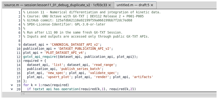
Open a GX-TXT Session and the integrated GNU Octave script editor. We will import the examples as Session scripts with distinct identifiers.
3. Numerical differentiation: what does it actually mean?
The derivative of a function describes its instantaneous rate of change with respect to a coordinate. If we have a continuous formula, we can sometimes differentiate it symbolically. If we have only a list of sampled values, we need to construct an approximation.
Between two consecutive points, the slope of the secant line is:
\[D_i^{\mathrm{forward}}=\frac{C_{i+1}-C_i}{t_{i+1}-t_i}\]
For interior points, another approximation uses the two neighbours of the point:
\[D_i^{\mathrm{centered}}\approx\frac{C_{i+1}-C_{i-1}}{t_{i+1}-t_{i-1}}\]
At the endpoints of the interval, there is no pair of points on both sides, so one-sided secants are used. This is the behaviour of the numerical kernel accessed through the GX-TXT service in this lesson.
3.1 Local derivative versus regression slope
Lesson 10 introduced linear regression, for example y = a + b*x. The coefficient b is a slope estimated from the set of observations, based on the chosen model and fitting criterion. In general, it is not the local derivative of a nonlinear curve.
A numerical derivative, by contrast, can return a different slope at each point. For our exponential decay, it is strongly negative at first and gradually approaches zero.
An example of interpretation
A line fitted to the entire kinetic curve provides a single average slope in the context of the fitting model. The derivative dC/dt, on the other hand, provides 101 local estimates, one for each sampled instant. They do not convey the same information.
3.2 Physical dimensions and sign
Because C is expressed in mmol/L and t in seconds, the derivative has units of mmol/(L·s). It is negative because the amount of substance is decreasing. If the phenomenon is expressed as a positive disappearance rate, we must explicitly define r(t) = -dC/dt.
The analytical model provides an independent reference:
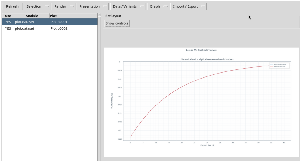
\[\frac{dC}{dt}=-kC_0e^{-kt}=-kC(t)\]
dcdt_exact = -rate_constant_s_inverse * concentration_mmol_L;
max_abs_derivative_error = max(abs(dcdt_numeric - dcdt_exact));
4. Numerical integration: area and accumulation
An integral does not describe a rate of change; it describes the total contribution of a quantity over an interval. For a positive concentration, the area under the curve is positive as well.
4.1 From summation to the trapezoidal rule
For sampled data, we approximate each segment of the curve between two points by a straight line. The corresponding area is that of a trapezoid:
\[A_i\approx\frac{C_i+C_{i+1}}{2}(t_{i+1}-t_i)\]
Adding all contributions gives the composite trapezoidal rule:
\[I(T)\approx\sum_{i=0}^{n-2}\frac{C_i+C_{i+1}}{2}(t_{i+1}-t_i)\]
The factor (t_(i+1)-t_i) is essential. If the intervals are different, using one width for every trapezoid would introduce a systematic error into the reconstructed area.
4.2 Definite integral versus cumulative integral
We may want to know only the integral over the full interval, or the accumulated quantity up to each instant:
\[I(T)=\int_{0}^{T}C(t)\,dt\qquad\text{and}\qquad I(t_i)=\int_0^{t_i}C(t)\,dt\]
| Result | Data shape | Scientific question |
|---|---|---|
| Total integral | One scalar | How much accumulated between 0 and 60 s? |
| Cumulative integral | A vector of 101 values | How much accumulated up to each instant? |
The cumulative mean in Lesson 09 was a mean calculated over an increasing number of observations. A cumulative integral is a different operation: it sums contributions weighted by the widths of the time intervals. In general, it is neither the simple sum of samples nor a running mean.
4.3 Units of the integral
Integrating a concentration with respect to time multiplies their units, giving mmol·s/L. The result is no longer a concentration or a dimensionless number. In an applied context it may represent concentration–time exposure, but its physical interpretation depends on how the experiment is defined.
For the chosen exponential kinetics, we also know the exact expression:
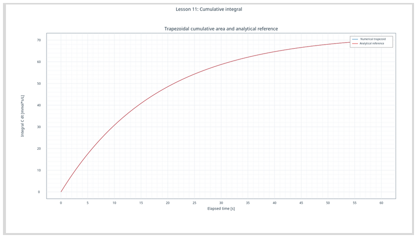
\[I(t)=\int_0^t C_0e^{-k\tau}\,d\tau=\frac{C_0}{k}\left(1-e^{-kt}\right)\]
area_exact = initial_concentration_mmol_L / rate_constant_s_inverse * ...
    (1 - exp(-rate_constant_s_inverse * time_s));
exact_total = area_exact(end);
5. Numerical accuracy: what are we actually measuring?
In Lesson 04, we encountered the error introduced when integrating a differential equation over time using Euler’s method. Here we encounter a different error from the same general family of numerical problems: discretization error, caused by reconstructing a derivative or an area from a finite set of points.
Comparison with the analytical solution allows us to measure this error without confusing it with sensor error or variation between observations:
\[E_D=\max_i\left|D_{\mathrm{numerical}}(t_i)-D_{\mathrm{exact}}(t_i)\right|\]
\[E_{I,\mathrm{rel}}=\frac{\left|I_{\mathrm{numerical}}(T)-I_{\mathrm{exact}}(T)\right|}{\left|I_{\mathrm{exact}}(T)\right|}\]
The relative-error formula requires a nonzero exact reference. This condition is satisfied in our experiment.
Three concepts not to confuse
Discretization error: the difference introduced by a numerical approximation on a finite grid. Experimental uncertainty: information about variability or limitations in measurements. Fitting residual: the difference between an observation and the value predicted by an estimated model, as in Lesson 10. None of these three quantities can automatically stand in for another.
5.1 Why is a finer grid not always the solution?
For smooth, noise-free data, increasing the sampling density usually reduces approximation error. Real experimental data, however, are not perfect. If a concentration measurement contains an error epsilon, the difference between two measurements also contains the difference between their errors:
\[\delta D_i\approx\frac{\varepsilon_{i+1}-\varepsilon_{i-1}}{t_{i+1}-t_{i-1}}\]
When the interval in the denominator decreases, the same noise can become much more prominent in the derivative. This is an important connection with the noisy signals studied in Lessons 07–09: differentiation tends to emphasize high-frequency noise, whereas integration often attenuates rapidly varying components through accumulation.
Filtering or regularizing the data may help, but it introduces additional choices and potential distortions. To keep these effects separate, this lesson uses a completely noise-free model.
6. Three new operations of the public Numeric API
NUMERIC_API_v1 is not a new private library. It is the public GX-TXT mathematical service already used in earlier lessons for arithmetic, statistics and fitting. In P008, the differentiation and integration operations are callable through the Octave Script Bridge.
The general call syntax is:
result = gxtxt_api_call(api_id, operation_name, arguments_cell);The first argument identifies the service, the second selects the operation, and the third is a cell array of positional arguments. The functions gxtxt_api_require and gxtxt_api_has_operation let us check dependencies before computation.
6.1 differentiate: deriving a sampled series
numeric_api = 'NUMERIC_API_v1';
gxtxt_api_require({numeric_api});
assert(gxtxt_api_has_operation(numeric_api, 'differentiate'));

derivative_result = gxtxt_api_call(numeric_api, 'differentiate', ...
    {time_s, concentration_mmol_L, struct()});
dcdt_numeric = derivative_result.dy_dx(:);
The API accepts x, y and an options structure. The vectors must have the same length and finite numeric values, with strictly increasing X coordinates. The returned structure contains x, dy_dx, n and method metadata. The dy_dx field contains the derivative vector.
Native GNU Octave functions remain useful for studying the mathematics: the actual differentiation kernel uses gradient(y,x). In the final script, however, we do not run a separate, disconnected numerical calculation: we call the public GX-TXT service and interpret its response.
6.2 integrate: definite integration
integral_result = gxtxt_api_call(numeric_api, 'integrate', ...
    {time_s, concentration_mmol_L, struct()});
area_total = integral_result.value;
This operation computes the trapezoidal integral over the entire grid and returns the scalar value, along with information such as the range and method. The corresponding Octave kernel is trapz(x,y).
6.3 cumulativeIntegrate: one integral at each instant
cumulative_result = gxtxt_api_call(numeric_api, 'cumulativeIntegrate', ...
    {time_s, concentration_mmol_L, struct()});
area_numeric = cumulative_result.integral(:);
assert(abs(area_numeric(end) - area_total) < 1e-8);
The result contains the x axis and an integral vector aligned with the original coordinates. The first integral value is zero; the last must agree with the definite integral within a declared tolerance. The corresponding numerical kernel in Octave is cumtrapz(x,y).
An important detail about the public operation name
The module’s mathematical documentation calls the operation cumulative_integrate, but the registered name callable through the P008 Octave Script Bridge is cumulativeIntegrate. For this reason the script checks and invokes exactly cumulativeIntegrate: the two strings are not interchangeable in the dispatcher.
7. Preparing and publishing the source Dataset
Start GX-TXT with a new Session. Open Viewers → Octave Scripts, import L11_00_Prepare_Kinetic_Decay.m, assign a distinct Script ID and save it. Run the Job through Run → Open Script Runner.
The script generates 101 time–concentration pairs, describes them with units and Variable IDs, and publishes them using DATASET_PUBLICATION_API_v2/publish_series_batch. A subsequent read using CANONICAL_DATASET_API_v2/read_range checks that the saved values match the generated values.
The source Dataset ID is lesson11_decay_observations; the X Variable ID is time_s, and the Y Variable ID is concentration_mmol_L. We do not need to open storage files or access the framework’s internal registries.
Script execution order
First: prepare and publish the Dataset. Second: explore the intentional error in the debugger. Third: execute the corrected calculation. All three scripts use the same canonical Dataset within the same Session, but they must have distinct Script IDs.
8. An intentional scientific error: two identical timestamps
The second script introduces an error into the time grid:
duplicate_time_s = time_s;
duplicate_time_s(32) = duplicate_time_s(31);
time_steps_s = diff(duplicate_time_s);
is_strictly_increasing = all(time_steps_s > 0);
zero_interval_count = sum(time_steps_s == 0);
The check all(time_steps_s > 0) now returns false, while zero_interval_count equals one. This is not a syntax error: the data violate a mathematical condition required by the algorithm.
Open Run → Debug Session script, set a breakpoint at line 35 of L11_01_Debug_Duplicate_Timestamp.m, where the API call occurs, and press Start Debug. While paused, inspect duplicate_time_s, time_steps_s and is_strictly_increasing.
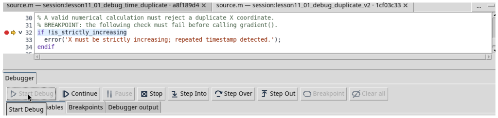
When we press Continue, the request reaches the numerical service and produces a documented error:
NUMERIC_API_v1/differentiate: math.numeric API v1:
X contains duplicate coordinate values
This time it is not the demonstration script that blocks the call in advance: the public Numeric API itself rejects the duplicated coordinate.
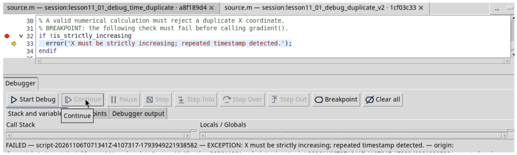
We do not automatically correct the data by sorting timestamps or deleting samples. Incorrect sorting could break the association between coordinates and measurements; deleting a point might remove valid experimental information. Corrections must follow an examination of the data source.
9. Running the corrected solution
Import L11_02_Calculus_Correct.m, save it with a third Script ID, and execute it through the Script Runner. The script reads the original Dataset, rejects nonfinite values and grids that are not strictly increasing, checks for nonuniform sampling and invokes the three public numerical operations.
After computing the results, it compares derivatives and integrals with the known analytical expressions, applies explicit validation tolerances and publishes four new Datasets in a single atomic transaction.

9.1 Numerical results and interpretation
| Quantity | Value | Meaning |
|---|---|---|
| Total numerical integral | 70.05013189 mmol·s/L | Trapezoidal area over the full interval |
| Analytical integral | 70.04486055 mmol·s/L | Exact value for the exponential model |
| Relative integral error | 0.0075266% | Relative difference from the analytical reference |
| Maximum absolute derivative error | 0.00057431 mmol/(L·s) | Largest pointwise difference from the exact derivative |
The trapezoidal rule produces a slightly larger integral than the exact result for this smooth, convex, decreasing exponential curve. This does not mean that the API “adds extra concentration”: the result depends on the geometric approximation, the step sizes and the curvature of the function.

10. Visualizing the derivative and integral in GX-TXT
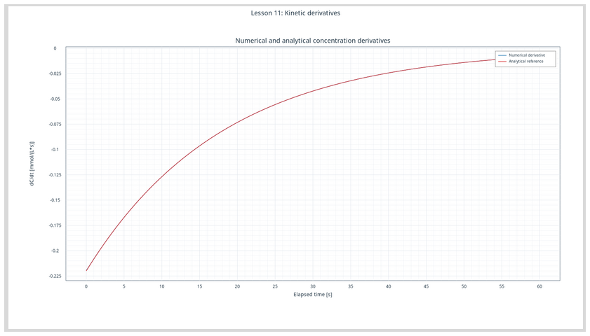
Numerical computation does not end with simply printing values. GX-TXT publishes four derived Datasets, each with coordinates, units, metadata and provenance. Their names are:
| Dataset ID | Quantity | Y unit |
|---|---|---|
lesson11_derivative_numeric | Numerical derivative | mmol/(L·s) |
lesson11_derivative_analytic | Analytical derivative | mmol/(L·s) |
lesson11_integral_cumulative | Numerical cumulative integral | mmol·s/L |
lesson11_integral_analytic | Analytical cumulative integral | mmol·s/L |
The first graph compares two derivatives: both are negative and approach zero as the concentration decreases. The difference is small relative to the scale of the curves, but it can still be quantified point by point.
The second graph shows the cumulative integrals: they increase over time because concentration remains positive. The final value of the numerical curve agrees with the total integral returned by integrate within the specified tolerance.
11. How the script connects Octave to GX-TXT APIs
We encountered the reading, publication and plotting APIs in Lessons 05–10. Here we reuse them without repeating all their contracts, focusing instead on each service’s responsibility.
| Public API | Operations used | Responsibility |
|---|---|---|
OCTAVE_SCRIPT_BRIDGE_API_v1 | gxtxt_api_require, gxtxt_api_has_operation, gxtxt_api_call | Check and invoke registered services |
CANONICAL_DATASET_API_v2 | list, read_range | Read Datasets and variables through stable identifiers |
NUMERIC_API_v1 | differentiate, integrate, cumulativeIntegrate | Perform scientific differentiation and integration |
DATASET_PUBLICATION_API_v2 | publish_series_batch | Atomically publish derived Datasets |
PLOT_DATASET_API_v4 | new_spec, validate_spec, upsert_plot, render, artifacts | Register and display persistent plots linked to Datasets |
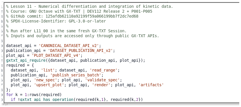
The central mathematical part of the corrected script is short:
derivative_result = gxtxt_api_call(numeric_api, 'differentiate', ...
    {time_s, concentration_mmol_L, struct()});

cumulative_result = gxtxt_api_call(numeric_api, 'cumulativeIntegrate', ...
    {time_s, concentration_mmol_L, struct()});

integral_result = gxtxt_api_call(numeric_api, 'integrate', ...
    {time_s, concentration_mmol_L, struct()});

dcdt_numeric = derivative_result.dy_dx(:);
area_numeric = cumulative_result.integral(:);
area_total = integral_result.value;
The three results have different shapes: the first provides a vector of derivatives, the second a vector of running integrals, and the third a single scalar. Octave structures also carry information about the numerical method; we must not assume that every response is directly a vector.
11.1 Why register a PlotSpec instead of using plot()?
Octave’s native plotting function is useful for learning the language, but here we want a scientific representation that remains traceable to published results. Using Plot Dataset, we explicitly define axes, units, Dataset IDs and Variable IDs. The graph therefore remains a persistent resource in the GX-TXT Session.
The method learned in Lesson 08 still applies: new_spec creates the specification, validate_spec checks it, upsert_plot registers the variant, render requests visualization, and artifacts returns references to the generated artifacts.
12. Common errors and essential checks
- No open Session: the Script Bridge works within GX-TXT’s execution context, not as a substitute for an ordinary Octave terminal.
- Missing source Dataset: run
L11_00_Prepare_Kinetic_Decay.mfirst. - Duplicate or disordered X coordinates: inspect
diff(time_s); the numerical service requires a valid grid. - Cumulative operation not found: use
cumulativeIntegratewith the internal capital letter when calling through the Bridge. - Output IDs already exist: repeat the experiment in a new Session; do not delete internal files directly.
- The derivative is very noisy: before applying a filter, consider time resolution, measurement noise and the physical meaning of the operation.
- Plots do not appear: check canonical identifiers and validate the PlotSpec before rendering it.
13. Suggested exercises
- Reduce the number of samples from 101 to 51. Compare the maximum derivative error and the relative integral error: what change do you observe, and why?
- Set the exponent used to generate time coordinates to 1.0, obtaining a uniform grid. Adjust the teaching check for nonuniform sampling and repeat the calculations without changing the numerical API names.
- Increase the rate constant to 0.10 s⁻¹, updating both curve generation and the analytical reference solution. Check the sign and order of magnitude of the new derivative.
- Calculate a series for the positive disappearance rate
-dcdt_numeric. Define a consistent Variable ID and physical unit before publishing it. - Add synthetic noise with a known standard deviation. Compare the sensitivity of the derivative and cumulative integral, without presenting the numerical difference as an estimate of experimental uncertainty.
- Investigate why the first and last derivative samples may have different errors from interior samples. Repeat the comparison excluding the endpoints from the comparison only, without modifying the original Datasets.
14. Lesson materials and references
The three GNU Octave scripts distributed with this article are:
L11_00_Prepare_Kinetic_Decay.m: generates and publishes the synthetic kinetic curve.L11_01_Debug_Duplicate_Timestamp.m: deliberately triggers a coordinate error for debugging.L11_02_Calculus_Correct.m: performs the correct calculation using public numeric APIs, publishes the derived Datasets and creates persistent graphs.
All script comments are in English. The examples are distributed under GNU GPL v3 or later.
GX-TXT reference version
Framework 0.9.8.10-dev-112 Release 2, cumulative patch P008. Official distribution: GX-TXT DEV112-r2 P008 on GitHub. The patch source bundle identifies commit f691b0f6e1016cb9af3db30ba3d1c8b5ea91429c; the GitHub release tag points to 17ff2a7f93de0612015a873e626f87dbeb56b6a2. API contract versions are independent of the framework release number.
Public documentation references:
- Octave Script Bridge API v1
- Numeric API v1
- Canonical Dataset API v2
- Dataset Publication API v2
- Plot Dataset API v4
15. Complete GNU Octave scripts
To view or copy the scripts without making the page excessively long, the three complete source files are available in the expandable sections below.
L11_00_Prepare_Kinetic_Decay.m — Preparing and publishing the source Dataset
% Lesson 11 - Create a synthetic first-order kinetic decay Dataset.
% Course: GNU Octave with GX-TXT | DEV112 Release 2 + P008
% GitHub release: https://github.com/giuxlab-hub/GX-TXT/releases/tag/v0.9.8.10-dev-112-r2-p008
% P008 source commit (release bundle): f691b0f6e1016cb9af3db30ba3d1c8b5ea91429c
% SPDX-License-Identifier: GPL-3.0-or-later
%
% Run once in a fresh GX-TXT Session with the managed Octave Script Workspace.
% These are synthetic, noise-free observations, not laboratory measurements.

dataset_api = 'CANONICAL_DATASET_API_v2';
publication_api = 'DATASET_PUBLICATION_API_v2';
gxtxt_api_require({dataset_api, publication_api});
assert(gxtxt_api_has_operation(dataset_api, 'list'));
assert(gxtxt_api_has_operation(dataset_api, 'read_range'));
assert(gxtxt_api_has_operation(publication_api, 'publish_series_batch'));

% A nonlinear time transformation creates an ascending, nonuniform grid.
sample_count = 101;
time_s = 60 * (linspace(0, 1, sample_count)' .^ 1.4);
initial_concentration_mmol_L = 4.0;
rate_constant_s_inverse = 0.055;
concentration_mmol_L = initial_concentration_mmol_L * ...
    exp(-rate_constant_s_inverse * time_s);
assert(all(diff(time_s) > 0));
assert(all(isfinite(concentration_mmol_L)));
assert(time_s(1) == 0 && abs(time_s(end)-60) < 1e-12);

source_id = 'lesson11_decay_observations';
present = gxtxt_api_call(dataset_api, 'list', {});
if any(strcmp(present, source_id))
  error('Source Dataset already exists. Create a fresh Session.');
endif

x_variable = struct('variable_id', 'time_s', 'name', 'time_s', ...
  'display_label', 'Elapsed time', 'unit', 's', 'dtype', 'float64', ...
  'value_kind', 'number', 'semantic_role', 'time', ...
  'semantic_source', 'generator');
y_variable = struct('variable_id', 'concentration_mmol_L', ...
  'name', 'concentration_mmol_L', ...
  'display_label', 'Synthetic concentration', 'unit', 'mmol/L', ...
  'dtype', 'float64', 'value_kind', 'number', ...
  'semantic_source', 'generator');

meta = struct();
meta.('simulation.synthetic') = true;
meta.('simulation.kinetic_order') = 1;
meta.('simulation.initial_concentration_mmol_L') = initial_concentration_mmol_L;
meta.('simulation.rate_constant_s_inverse') = rate_constant_s_inverse;
meta.('simulation.nonuniform_sampling') = true;
request = struct('dataset_id', source_id, 'contract', 'table.generic', ...
  'storage', 'auto', 'x_values', time_s, ...
  'y_values', concentration_mmol_L, 'x_variable', x_variable, ...
  'y_variable', y_variable, 'producer_version', '1.0.0', ...
  'source', 'GX-TXT GNU Octave Lesson 11', ...
  'provenance', 'Deterministic synthetic first-order decay', ...
  'notes', 'Nonuniform ascending time grid, noise-free concentrations', ...
  'structured_metadata', meta);
batch = struct('series', {{request}});
receipt = gxtxt_api_call(publication_api, 'publish_series_batch', {batch});
if !receipt.atomic || receipt.output_count != 1
  error('The public publication receipt is not confirmed.');
endif

recovered = gxtxt_api_call(dataset_api, 'read_range', ...
  {source_id, {'time_s', 'concentration_mmol_L'}, 0, sample_count});
assert(max(abs(recovered.time_s.values(:)-time_s)) < 1e-10);
assert(max(abs(recovered.concentration_mmol_L.values(:)-concentration_mmol_L)) < 1e-10);
fprintf('PASS: published %d synthetic kinetic samples as %s.\n', ...
        sample_count, source_id);
L11_01_Debug_Duplicate_Timestamp.m — Intentional error and derivative debugging
% Lesson 11 - Intentional numerical-calculus error for the native debugger.
% Course: GNU Octave with GX-TXT | DEV112 Release 2 + P008
% GitHub release: https://github.com/giuxlab-hub/GX-TXT/releases/tag/v0.9.8.10-dev-112-r2-p008
% P008 source commit (release bundle): f691b0f6e1016cb9af3db30ba3d1c8b5ea91429c
% SPDX-License-Identifier: GPL-3.0-or-later
%
% Run after L11_00. Set a breakpoint immediately before the Numeric API call.
% Inspect duplicate_time_s, time_steps_s, and is_strictly_increasing.
% This script is expected to FAIL inside the public Numeric API, without publishing.

dataset_api = 'CANONICAL_DATASET_API_v2';
numeric_api = 'NUMERIC_API_v1';
gxtxt_api_require({dataset_api, numeric_api});
assert(gxtxt_api_has_operation(dataset_api, 'read_range'));
assert(gxtxt_api_has_operation(numeric_api, 'differentiate'));
observations = gxtxt_api_call(dataset_api, 'read_range', ...
  {'lesson11_decay_observations', {'time_s', 'concentration_mmol_L'}, 0, 101});
time_s = observations.time_s.values(:);
concentration_mmol_L = observations.concentration_mmol_L.values(:);
assert(numel(time_s) == 101 && numel(concentration_mmol_L) == 101);

% INTENTIONAL BUG: one sample repeats the previous timestamp.
% The time order is no longer strictly increasing: public Numeric API must reject it.
duplicate_time_s = time_s;
duplicate_time_s(32) = duplicate_time_s(31);
time_steps_s = diff(duplicate_time_s);
is_strictly_increasing = all(time_steps_s > 0);
zero_interval_count = sum(time_steps_s == 0);
fprintf('Strictly increasing = %d; repeated intervals = %d.\n', ...
        is_strictly_increasing, zero_interval_count);

% BREAKPOINT: inspect duplicate_time_s, time_steps_s and the false flag.
% The Numeric API itself rejects duplicate timestamps; no silent repair.
fprintf('Calling the public GX-TXT derivative with an invalid time grid.\n');
invalid_result = gxtxt_api_call(numeric_api, 'differentiate', ...
    {duplicate_time_s, concentration_mmol_L, struct()});
error('Unexpected success: the Numeric API accepted a duplicate timestamp.');
L11_02_Calculus_Correct.m — Numerical calculation with GX-TXT APIs, Dataset publication and plots
% Lesson 11 - Numerical differentiation and integration of kinetic data.
% Course: GNU Octave with GX-TXT | DEV112 Release 2 + P008
% GitHub release: https://github.com/giuxlab-hub/GX-TXT/releases/tag/v0.9.8.10-dev-112-r2-p008
% P008 source commit (release bundle): f691b0f6e1016cb9af3db30ba3d1c8b5ea91429c
% SPDX-License-Identifier: GPL-3.0-or-later
%
% Run after L11_00 in the same fresh GX-TXT Session.
% Inputs and outputs are accessed only through public GX-TXT APIs.

dataset_api = 'CANONICAL_DATASET_API_v2';
publication_api = 'DATASET_PUBLICATION_API_v2';
plot_api = 'PLOT_DATASET_API_v4';
numeric_api = 'NUMERIC_API_v1';
gxtxt_api_require({dataset_api, publication_api, plot_api, numeric_api});
required = {
  numeric_api, 'differentiate'; numeric_api, 'integrate';
  numeric_api, 'cumulativeIntegrate';
  dataset_api, 'list'; dataset_api, 'read_range';
  publication_api, 'publish_series_batch';
  plot_api, 'new_spec'; plot_api, 'validate_spec';
  plot_api, 'upsert_plot'; plot_api, 'render'; plot_api, 'artifacts'
};
for k = 1:rows(required)
  if !gxtxt_api_has_operation(required{k,1}, required{k,2})
    error('Missing public operation: %s/%s', required{k,1}, required{k,2});
  endif
endfor

% 1. Read the canonical observations by stable Variable ID.
source_id = 'lesson11_decay_observations';
present = gxtxt_api_call(dataset_api, 'list', {});
if !any(strcmp(present, source_id))
  error('Run L11_00 first in this fresh Session.');
endif
observations = gxtxt_api_call(dataset_api, 'read_range', ...
  {source_id, {'time_s', 'concentration_mmol_L'}, 0, 101});
time_s = observations.time_s.values(:);
concentration_mmol_L = observations.concentration_mmol_L.values(:);
n = numel(time_s);
if n != 101 || numel(concentration_mmol_L) != n || ...
  !all(isfinite(time_s)) || !all(isfinite(concentration_mmol_L)) || ...
  !all(diff(time_s) > 0)
  error('Invalid source data: a finite strictly increasing time grid is required.');
endif

% 2. Inspect the nonuniform grid using standard Octave vector operations.
time_steps_s = diff(time_s);
if max(time_steps_s) - min(time_steps_s) < 1e-8
  error('This experiment requires nonuniform sampling.');
endif

% 3. Use the public GX-TXT numerical CORE, not independent Octave kernels.
% NUMERIC_API_v1/differentiate returns x, dy_dx and method metadata.
derivative_result = gxtxt_api_call(numeric_api, 'differentiate', ...
  {time_s, concentration_mmol_L, struct()});
dcdt_numeric = derivative_result.dy_dx(:);

% The Script Bridge exposes cumulativeIntegrate (camelCase).
% The public Numeric contract describes this as cumulative_integrate.
cumulative_result = gxtxt_api_call(numeric_api, 'cumulativeIntegrate', ...
  {time_s, concentration_mmol_L, struct()});
area_numeric = cumulative_result.integral(:);

% Integrate evaluates the entire range and returns its scalar value.
integral_result = gxtxt_api_call(numeric_api, 'integrate', ...
  {time_s, concentration_mmol_L, struct()});
area_total = integral_result.value;
assert(numel(dcdt_numeric) == n && numel(area_numeric) == n);
assert(all(isfinite(dcdt_numeric)) && all(isfinite(area_numeric)));
assert(isfinite(area_total) && area_total > 0);
assert(max(abs(derivative_result.x(:)-time_s)) < 1e-10);
assert(max(abs(cumulative_result.x(:)-time_s)) < 1e-10);
assert(abs(area_numeric(end) - area_total) < 1e-8);

% 4. Compare with the analytical first-order kinetic reference.
rate_constant_s_inverse = 0.055;
initial_concentration_mmol_L = 4.0;
dcdt_exact = -rate_constant_s_inverse * concentration_mmol_L;
area_exact = initial_concentration_mmol_L / rate_constant_s_inverse * ...
    (1 - exp(-rate_constant_s_inverse * time_s));
exact_total = area_exact(end);
max_abs_derivative_error = max(abs(dcdt_numeric - dcdt_exact));
max_abs_integral_error = max(abs(area_numeric - area_exact));
relative_total_error = abs(area_total - exact_total) / exact_total;
fprintf('Time intervals: minimum %.6f s, maximum %.6f s.\n', ...
        min(diff(time_s)), max(diff(time_s)));
fprintf('Total numerical exposure: %.8f mmol*s/L.\n', area_total);
fprintf('Exact integrated exposure: %.8f mmol*s/L.\n', exact_total);
fprintf('Relative integral error: %.8g.\n', relative_total_error);
fprintf('Max derivative absolute error: %.8g mmol/(L*s).\n', ...
        max_abs_derivative_error);
fprintf('GX-TXT derivative method: %s; integral method: %s.\n', ...
        derivative_result.method, integral_result.method);
if relative_total_error > 0.002 || max_abs_derivative_error > 0.003
  error('Numerical calculus accuracy exceeds lesson tolerance.');
endif

% 5. Publish four scientific series with the true physical dimensions.
derived_ids = {
  'lesson11_derivative_numeric',
  'lesson11_derivative_analytic',
  'lesson11_integral_cumulative',
  'lesson11_integral_analytic'
};
for k = 1:numel(derived_ids)
  if any(strcmp(present, derived_ids{k}))
    error('Output exists: %s. Use a fresh Session.', derived_ids{k});
  endif
endfor
x_variable = struct('variable_id', 'time_s', 'name', 'time_s', ...
  'display_label', 'Elapsed time', 'unit', 's', 'dtype', 'float64', ...
  'value_kind', 'number', 'semantic_role', 'time', ...
  'semantic_source', 'plugin');
rate_variable = struct('variable_id', 'dcdt_mmol_L_s', ...
  'name', 'dcdt_mmol_L_s', 'display_label', 'Concentration derivative', ...
  'unit', 'mmol/(L*s)', 'dtype', 'float64', ...
  'value_kind', 'number', 'semantic_source', 'plugin');
area_variable = struct('variable_id', 'area_mmol_s_L', ...
  'name', 'area_mmol_s_L', 'display_label', 'Cumulative concentration-time integral', ...
  'unit', 'mmol*s/L', 'dtype', 'float64', ...
  'value_kind', 'number', 'semantic_source', 'plugin');
y_values = {dcdt_numeric, dcdt_exact, area_numeric, area_exact};
y_variables = {rate_variable, rate_variable, area_variable, area_variable};
descriptions = {'GX-TXT Numeric API finite-difference derivative', ...
  'Analytical derivative', 'GX-TXT Numeric API cumulative trapezoid', ...
  'Analytical definite integral'};
series = cell(1, numel(derived_ids));
for k = 1:numel(derived_ids)
  metadata = struct();
  metadata.('analysis.method') = descriptions{k};
  metadata.('analysis.source_dataset_id') = source_id;
  metadata.('analysis.nonuniform_grid') = true;
  metadata.('analysis.synthetic_input') = true;
  series{k} = struct('dataset_id', derived_ids{k}, ...
    'contract', 'table.generic', 'storage', 'auto', ...
    'x_values', time_s, 'y_values', y_values{k}, ...
    'x_variable', x_variable, 'y_variable', y_variables{k}, ...
    'producer_version', '1.0.0', ...
    'source', 'GX-TXT GNU Octave Lesson 11', ...
    'source_dataset_ids', {{source_id}}, ...
    'provenance', 'Public GX-TXT NUMERIC_API_v1 calculus on canonical GX-TXT synthetic kinetic data', ...
    'notes', descriptions{k}, 'structured_metadata', metadata);
endfor
batch = struct('series', {series});
receipt = gxtxt_api_call(publication_api, 'publish_series_batch', {batch});
if !receipt.atomic || receipt.output_count != 4
  error('Expected atomic receipt for four derived Datasets.');
endif

% 6. Verify all published values through the canonical public Dataset reader.
for k = 1:numel(derived_ids)
  recovered = gxtxt_api_call(dataset_api, 'read_range', ...
    {derived_ids{k}, {'time_s', y_variables{k}.variable_id}, 0, n});
  saved = recovered.(y_variables{k}.variable_id).values(:);
  assert(numel(saved) == n);
  assert(max(abs(saved - y_values{k})) < 1e-9);
endfor

% 7. Two native, persistent plots preserve Dataset and Variable IDs.
derivative_plot = gxtxt_api_call(plot_api, 'new_spec', ...
  {'plot.dataset.xy', 'Lesson 11: Kinetic derivatives'});
dp = derivative_plot.panels{1};
dp.id = 'derivatives';
dp.title = 'Numerical and analytical concentration derivatives';
dp.axes = struct('x', struct('label', 'Elapsed time [s]', 'scale', 'linear'), ...
  'y_left', struct('label', 'dC/dt [mmol/(L*s)]', 'scale', 'linear'));
dp.series = {
  struct('id', 'numerical', 'label', 'Numerical derivative', ...
    'dataset_id', derived_ids{1}, 'x_variable_id', 'time_s', ...
    'y_variable_id', 'dcdt_mmol_L_s', 'axis', 'left', 'kind', 'line'),
  struct('id', 'analytic', 'label', 'Analytical reference', ...
    'dataset_id', derived_ids{2}, 'x_variable_id', 'time_s', ...
    'y_variable_id', 'dcdt_mmol_L_s', 'axis', 'left', 'kind', 'line')
};
derivative_plot.panels = {dp};
if !gxtxt_api_call(plot_api, 'validate_spec', {derivative_plot})
  error('Numerical derivative PlotSpec invalid.');
endif
derivative_ref = gxtxt_api_call(plot_api, 'upsert_plot', ...
  {'lesson11_kinetic_derivatives', derivative_plot});
gxtxt_api_call(plot_api, 'render', {derivative_ref});
derivative_artifacts = gxtxt_api_call(plot_api, 'artifacts', {derivative_ref});

area_plot = gxtxt_api_call(plot_api, 'new_spec', ...
  {'plot.dataset.xy', 'Lesson 11: Cumulative integral'});
ap = area_plot.panels{1};
ap.id = 'integrals';
ap.title = 'Trapezoidal cumulative area and analytical reference';
ap.axes = struct('x', struct('label', 'Elapsed time [s]', 'scale', 'linear'), ...
  'y_left', struct('label', 'Integral C dt [mmol*s/L]', 'scale', 'linear'));
ap.series = {
  struct('id', 'numerical', 'label', 'Numerical trapezoid', ...
    'dataset_id', derived_ids{3}, 'x_variable_id', 'time_s', ...
    'y_variable_id', 'area_mmol_s_L', 'axis', 'left', 'kind', 'line'),
  struct('id', 'analytic', 'label', 'Analytical reference', ...
    'dataset_id', derived_ids{4}, 'x_variable_id', 'time_s', ...
    'y_variable_id', 'area_mmol_s_L', 'axis', 'left', 'kind', 'line')
};
area_plot.panels = {ap};
if !gxtxt_api_call(plot_api, 'validate_spec', {area_plot})
  error('Numerical integration PlotSpec invalid.');
endif
area_ref = gxtxt_api_call(plot_api, 'upsert_plot', ...
  {'lesson11_kinetic_integral', area_plot});
gxtxt_api_call(plot_api, 'render', {area_ref});
area_artifacts = gxtxt_api_call(plot_api, 'artifacts', {area_ref});
fprintf('PASS: public NUMERIC_API_v1 calculus, 4 derived Datasets, 2 native plots, read-back verified.\n');
disp(derivative_artifacts);
disp(area_artifacts);
This exercise concludes our work on numerical derivatives and integrals and prepares us to use computational methods in more advanced applications, where the choice of grid, units and numerical model is an integral part of scientific interpretation.
Other steps of this project
- Lesson 01 — Your First GNU Octave Script in GX-TXT
- Lesson 02 — Variables, Data Types and Operators in GNU Octave with GX-TXT
- Lesson 03 — Vectors and Matrices in GNU Octave with GX-TXT: Temperature Measurement Analysis
- Lesson 04 — Conditions, Loops, and Functions. Simulating Newton’s Law of Cooling
- Lesson 05: Scientific Datasets and Variable IDs
- Lesson 06 — Selecting and Reading Experimental Data with GNU Octave and GX-TXT