

Lesson 15 — RLC Circuits and Bode Diagrams with GNU Octave and GX-TXT
An electrical circuit provides a concrete example of why complex numbers are essential to scientific computing. In this lesson we simulate a series RLC circuit, calculate its sinusoidal frequency response, derive magnitude and phase Bode diagrams, and learn how the Octave debugger can reveal a units error. Scientific results are published and visualized within GX-TXT using its public APIs exclusively.
Learning goals and prerequisites
By the end of this lesson, we will be able to construct logarithmically spaced vectors, represent impedances with complex numbers, perform element-wise operations, convert voltage-amplitude ratios into decibels, calculate phase in degrees, and verify a numerical result against an independent analytical model. We draw on vectors and matrices (Lesson 03), functions and checks (Lesson 04), Datasets (Lessons 05–07), scientific plots (Lesson 08), debugging (Lessons 09–14), and complex numbers in numerical analysis.
Connections with the first fourteen lessons
Lessons 01–04 introduced the Script Bridge, data types, complex numbers, vectors, and operators. Lessons 05–08 covered Dataset identification, reading, publication, and visualization; Lessons 09–12 added scientific checks, residual analysis, and linear algebra. In Lesson 13, we examined the magnitude and phase of FFT coefficients; in Lesson 14, we solved differential equations in the time domain.
| Previously studied concept | New scientific meaning in Lesson 15 |
|---|---|
Complex numbers and 1i (02, 12–13) |
Phasors and electrical impedances |
| Vectors and element-wise operations (02–03) | Circuit response calculated at many frequencies |
abs and angle on FFT coefficients (13) |
Magnitude and phase of an output/input ratio |
| Differential equations (04, 14) | Sinusoidal steady state rather than a transient |
| Debugger and numerical checks (08–14) | Physical units error that does not produce a syntax error |
| Canonical Datasets and Plot Dataset v4 (05–12) | Persistent Bode diagrams with logarithmic frequency axes |
The new problem is not how to write a vector. It is the transition from physical laws in time to a complex-valued function of frequency.
The circuit: R, L, and C in series
We connect a resistor \(R\), an inductor \(L\), and a capacitor \(C\) in series. We apply a sinusoidal voltage and take the voltage across the resistor as the output. This is essential: measuring voltage across the capacitor or inductor would produce a different transfer function.
| Physical quantity | Value | Unit |
|---|---|---|
| Resistance \(R\) | 20 | \(\Omega\) |
| Inductance \(L\) | 10 | mH |
| Capacitance \(C\) | 1 | \(\mu\mathrm{F}\) |
| Frequency range | 100–31,623 | Hz |
| Samples | 402, including \(f_0\) | — |
We assume ideal components, an ideal voltage source, and sinusoidal steady state. The model excludes coil winding resistance, dielectric losses, parasitic capacitances, and uncertainty in component values.
Why does this behave like a band-pass filter?
At very low frequencies, the capacitor has a large reactance magnitude. Little current flows through the series branch, and the resistor voltage is small. At very high frequencies, the inductor opposes changes in current and the resistor voltage again decreases. Between these extremes, there is a frequency where the two reactances cancel: series current is maximum and, for the ideal circuit, the resistor voltage reaches the input voltage.
This result depends on choosing the resistor as the output. Measuring across \(L\) or \(C\) would yield a different transfer function. Polarity matters as well: reversing the resistor-output terminals changes the sign of the complex ratio and shifts its phase by 180°, but leaves its magnitude unchanged.
Complex impedance and transfer function
Impedance is a complex quantity. GNU Octave represents the imaginary unit \(j\) using 1i. For angular frequency \(\omega=2\pi f\), the three impedances are
\[ Z_R=R,\qquad Z_L=j\omega L,\qquad Z_C=\frac{1}{j\omega C}. \]
Their sum is
\[ Z_{\mathrm{tot}}=R+j\left(\omega L-\frac{1}{\omega C}\right). \]
Because the same current flows through each element, the ratio between resistor output voltage and applied input voltage is
\[ H(j\omega)=\frac{V_R}{V_{\mathrm{in}}} =\frac{R}{R+j\bigl(\omega L-1/(\omega C)\bigr)}. \]
The magnitude \(|H|\) is a voltage-amplitude ratio, not a power ratio. Since the resistance is positive and reactive terms cancel at resonance, \(|H|\leq 1\): with the stated output terminals, this is a band-pass response.
From sinusoidal signals to phasors
Lesson 13 introduced the phase of Fourier coefficients. Here we introduce a phasor, a complex number representing the amplitude and phase of one sinusoid at a fixed frequency. Using the time convention \(e^{j\omega t}\), we write
\[ v(t)=\operatorname{Re}\!\left\{\widehat V e^{j\omega t}\right\},\qquad i(t)=\operatorname{Re}\!\left\{\widehat I e^{j\omega t}\right\}. \]
The phasors \(\widehat V\) and \(\widehat I\) are not samples in time. With this convention, taking a time derivative corresponds to multiplying a phasor by \(j\omega\):
\[ \frac{d}{dt}\left(\widehat I e^{j\omega t}\right)=j\omega\widehat I e^{j\omega t}. \]
From the inductor law \(v_L=L\,di/dt\) and the capacitor law \(i_C=C\,dv_C/dt\), we obtain \(\widehat V_L=j\omega L\widehat I\) and \(\widehat V_C=\widehat I/(j\omega C)\). A differential relation has become an algebraic one. This transition is valid for sinusoidal steady state, not for the initial switching transient.
Impedances are measured in ohms. The values must be converted first: \(10\,\mathrm{mH}=0.010\,\mathrm{H}\) and \(1\,\mu\mathrm{F}=10^{-6}\,\mathrm{F}\). Indeed, \(\omega L\), with \(\omega\) in radians per second, has units of ohms, and so does \(1/(\omega C)\). Correct units are a scientific check independent of Octave syntax.
Deriving rather than memorizing the transfer function
Kirchhoff’s voltage law gives \(\widehat V_{\mathrm{in}}=\widehat I(Z_R+Z_L+Z_C)\). The voltage across the resistor is \(\widehat V_R=\widehat I R\). Dividing the equations gives
\[ H(j\omega)=\frac{\widehat V_R}{\widehat V_{\mathrm{in}}} =\frac{R}{R+jX(\omega)},\qquad X(\omega)=\omega L-\frac{1}{\omega C}. \]
A transfer function is a ratio between two phasors at the same frequency: its magnitude gives the amplitude ratio and its argument gives the output phase relative to the input. Writing the net reactance as a real quantity \(X\) also gives an independent analytical check:
\[ |H|=\frac{R}{\sqrt{R^2+X^2}},\qquad \arg H=-\operatorname{atan2}(X,R). \]
The following values are theoretical calculations, not physical measurements:
| Frequency | Reactance \(X\) | \(|H|\) | Gain | Phase |
|---|---|---|---|---|
| 1,000 Hz | \(-96.32\,\Omega\) | 0.2033 | −13.84 dB | +78.27° |
| 1,591.549 Hz | \(0\,\Omega\) | 1.0000 | 0 dB | 0° |
| 2,500 Hz | \(+93.42\,\Omega\) | 0.2093 | −13.58 dB | −77.92° |
Phase is positive below resonance, where the net reactance is capacitive, and negative above resonance, where the net reactance is inductive. The sign change has a physical cause; it is not a graph-formatting choice.
Complex numbers, vectorization, and a logarithmic axis
In GNU Octave, we generate a vector using logspace and transpose it into a column. We insert the exact resonance frequency in the grid so the largest sampled result is not confused with the theoretical maximum.
R = 20;
L = 10e-3;
C = 1e-6;
f0 = 1/(2*pi*sqrt(L*C));
frequency_hz = sort([logspace(2,4.5,401)';f0]);
omega = 2*pi*frequency_hz;
z_total = R + 1i*omega*L + 1./(1i*omega*C);
H = R ./ z_total;
The ./ operator performs element-wise division: each frequency produces its own impedance and transfer value. The / operator can denote matrix division and is not interchangeable with ./. Similarly, .^ denotes an element-wise power.
The frequencies are logarithmically spaced. The graphical distance between 100 and 1,000 Hz is the same as that between 1,000 and 10,000 Hz. logspace defines where we evaluate the model; the Plot Dataset option scale='log' defines how we display those frequencies. The operations are distinct.
Logarithmic frequency sampling, instruction by instruction
logspace(2,4.5,401) produces 401 values between \(10^2\) and \(10^{4.5}\) Hz, equally spaced in the logarithm, not in hertz. A decade is a tenfold change in frequency; our range covers 2.5 decades. The transpose ' creates a real column vector, square-bracket concatenation adds \(f_0\), and sort restores ascending order.
frequency_hz = sort([logspace(2,4.5,401)'; f0]);
assert(iscolumn(frequency_hz));
assert(numel(frequency_hz) == 402);
assert(all(diff(frequency_hz) > 0));
Including the analytically known resonance value prevents confusion between the maximum on a finite sampled grid and the exact physical maximum. Sampling determines where calculations occur; the GX-TXT Plot Dataset setting scale='log' determines how the results appear. Changing the display scale does not change Dataset values.
Why is the logarithmic coefficient 20, rather than 10?
A decibel expresses a ratio. A power ratio uses \(10\log_{10}(P_2/P_1)\); a voltage-amplitude ratio such as \(V_R/V_{\mathrm{in}}\) uses \(20\log_{10}|V_R/V_{\mathrm{in}}|\). The factor 20 is consistent with power being proportional to the squared voltage when the resistive reference is unchanged.
| Amplitude ratio | Gain in dB | Interpretation |
|---|---|---|
| 1 | 0 | Equal amplitudes |
| \(1/\sqrt 2\approx 0.7071\) | −3.0103 | Half power, unchanged resistive reference |
| 0.5 | −6.0206 | Half the voltage amplitude |
A negative gain in dB does not mean a negative voltage: it means attenuation. A magnitude Bode plot uses a logarithmic X-axis in hertz and a numerically linear Y-axis in decibels. The already-calculated decibel values must not be logarithmically transformed a second time.
FFT phase versus transfer-function phase
In Lesson 13, angle described the phase of an FFT coefficient. Here, \(\arg H=\arg\widehat V_R-\arg\widehat V_{\mathrm{in}}\) is a phase difference between output and input at the same frequency. The numerical function is the same, but the physical quantity is different.
angle returns radians. unwrap can remove artificial \(2\pi\) jumps between neighboring phase samples, but does not convert radians into degrees or correct an invalid physical model. For this ideal band-pass response, phase remains between +90° and −90° and never crosses a 360° discontinuity. Here unwrap is a general precaution, not the reason the phase curve is continuous.
Decibels, phase, and Bode diagrams
The transfer magnitude is computed with abs(H). For a voltage-amplitude ratio, a magnitude Bode diagram uses
\[ G_{\mathrm{dB}}(f)=20\log_{10}|H(j2\pi f)|. \]
Do not use \(10\log_{10}|H|\) here: 10 is the coefficient for power ratios; the connection to squared voltage amplitudes requires appropriate reference impedances.
The phase is the complex argument:
\[ \varphi(f)=\arg H(j2\pi f)\,\frac{180}{\pi}. \]
gain_linear = abs(H);
gain_db = 20*log10(gain_linear);
phase_deg = unwrap(angle(H))*180/pi;
angle returns radians. unwrap removes potential artificial \(2\pi\) jumps in sampled phase. In this example, the continuous phase crosses zero at resonance; conversion into degrees is still required.
Resonance frequency, bandwidth, and quality factor
At resonance, inductive and capacitive reactances cancel:
\[ f_0=\frac{1}{2\pi\sqrt{LC}}\approx1591.549\,\mathrm{Hz}. \]
At \(f_0\), the denominator of \(H\) is real. The ideal resistor-output magnitude is 1 (0 dB) and the phase is 0°. The quality factor for the series circuit is
\[ Q=\frac{1}{R}\sqrt{\frac{L}{C}}=5. \]
The −3.0103 dB cutoff frequencies satisfy \(|H|=1/\sqrt2\). For \(R,L,C>0\), their angular frequencies are
\[ \omega_1=\frac{-R+\sqrt{R^2+4L/C}}{2L},\qquad \omega_2=\frac{R+\sqrt{R^2+4L/C}}{2L}. \]
Thus, \(f_1\approx1440.332\,\mathrm{Hz}\), \(f_2\approx1758.642\,\mathrm{Hz}\), and \(\Delta f=f_2-f_1=R/(2\pi L)\approx318.310\,\mathrm{Hz}\). Phase is +45° at the lower cutoff and −45° at the upper one. Below resonance the series response is predominantly capacitive; above resonance, predominantly inductive.
Two independent consistency relations are
\[ \sqrt{f_1f_2}=f_0,\qquad Q=\frac{f_0}{\Delta f}. \]
These checks verify the circuit model regardless of the graphical presentation.
Deriving the half-power frequencies and interpreting Q
For the same resistive reference, dissipated power is proportional to \(|H|^2\). At the half-power frequencies, \(|H|^2=1/2\). Substituting the analytical magnitude equation gives
\[ \frac{R^2}{R^2+X^2}=\frac12 \quad\Longrightarrow\quad |X|=R. \]
Below resonance, \(X=-R\); above resonance, \(X=+R\). Solving these two equations in \(\omega\) produces the formulas for \(\omega_1\) and \(\omega_2\) given above. They are not arbitrary positions chosen on a graph. The bandwidth \(\Delta f=f_2-f_1\) must not be confused with \(f_0\).
The quality factor \(Q\) describes resonant selectivity. Its energetic interpretation compares the maximum energy temporarily stored in the reactive elements with the energy dissipated per cycle. For this ideal series circuit, \(Q=\omega_0 L/R=f_0/\Delta f\). Increasing \(R\) with \(L,C\) fixed widens the band and lowers \(Q\), while the ideal resistor-output peak remains 0 dB.
Far from resonance, the asymptotic slopes can be derived:
\[ f\ll f_0:\quad |H|\simeq R\omega C \quad(+20\,\mathrm{dB/decade}), \]
\[ f\gg f_0:\quad |H|\simeq\frac{R}{\omega L} \quad(-20\,\mathrm{dB/decade}). \]
Sufficiently far below resonance, a tenfold frequency increase raises gain by approximately 20 dB; far above resonance, it lowers gain by approximately 20 dB. These are asymptotes, not exact straight-line behavior close to the resonance peak.
First script: an independent analytical reference
L15_00_Prepare_RLC_Reference.m calculates gain and phase using real-valued analytical expressions that do not rely on the complex division performed by the final script:
\[ |H|=\frac{R}{\sqrt{R^2+(\omega L-1/(\omega C))^2}},\qquad \varphi=-\operatorname{atan2}\!\left(\omega L-\frac1{\omega C},R\right). \]
These results are not experimental measurements; they are synthetic analytical data. The script publishes two GX-TXT Datasets: gain in dB and phase in degrees. Both use the independent variable frequency_hz and scientific metadata describing R, L, C, and the origin of the data.
Why use different formulas for the reference?
Program 00 calculates magnitude with a square root and phase with atan2, using real-valued expressions. Program 02 instead uses complex division with abs and angle. Comparing mathematically equivalent formulas implemented in different ways is a stronger numerical check than repeating the exact same calculation twice.
This comparison tests numerical consistency, not experimental accuracy. Both scripts assume the same ideal circuit. We must distinguish correct syntax, correct mathematical implementation, and the physical appropriateness of the model; passing any one test does not guarantee the others.
Second script: debugging a phase-unit error
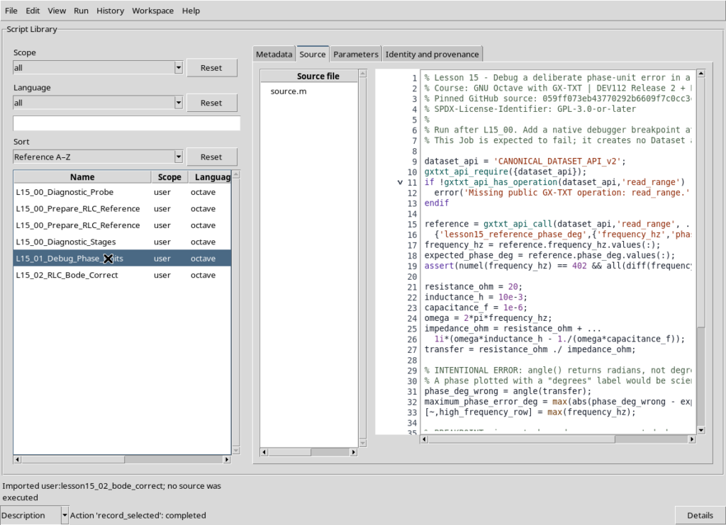
L15_01_Debug_Phase_Units.m reconstructs the correct transfer function but deliberately contains:
phase_deg_wrong = angle(transfer);Despite its name, the variable contains radians, not degrees. This error is particularly dangerous because the values are smooth and can be graphed: the program would not stop by itself. We compare the series with the analytical reference. Since the difference exceeds the chosen tolerance by a large margin, the Job ends with the expected GXTXT:Lesson15:PhaseUnits error.
From Run → Debug Session script, place a breakpoint at the BREAKPOINT comment. Inspect phase_deg_wrong, expected_phase_deg, maximum_phase_error_deg, and the frequency of the final sample. Selecting Continue triggers the scientific validation check. This failed Job is intentional and is not a defect in GX-TXT.
The debugger identifies an error in physical meaning
The number \(\pi/2\) is approximately 1.571 radians, but corresponds to 90 degrees. Assigning angle(transfer) to phase_deg_wrong produces smooth, drawable values with the wrong declared unit. A debugger lets us inspect the mismatch before the wrong results are published.
At the breakpoint, compare the two arrays at the same frequency index. First inspect their meanings and units, then their numerical sizes: near an expected phase of 90°, the incorrect value will be about 1.57. The correction is unwrap(angle(transfer))*180/pi, not a change to the plot’s Y-axis label. Changing the declared unit alone would hide the mistake rather than fix it.
The Job fails intentionally when numerical values are inconsistent with the units they are supposed to represent. This is an executable scientific check, analogous to the rank checks in Lesson 12 and mass conservation checks in Lesson 14.
Third script: the corrected result and independent validation
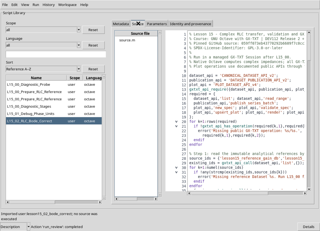
L15_02_RLC_Bode_Correct.m uses 1i, abs, angle, unwrap, log10, and vectorized operations to obtain the complex frequency response. It compares the result against the analytical Datasets using the maximum absolute error for gain in dB and phase in degrees. It also checks circuit passivity, phase behavior, resonance, and the relations between cutoff frequencies.
These checks detect errors that syntactic validation would miss: an inverted voltage ratio, a phase sign mistake, a missing radians-to-degrees conversion, or confusion between matrix and element-wise division.
The public GX-TXT APIs used in this lesson
GNU Octave calculates vectors, impedances, and mathematical quantities. GX-TXT manages Session-scoped scientific data, resource identities, publication, and persistent plots. None of the scripts opens framework-internal files directly.
| Public API or operation | Purpose and result |
|---|---|
gxtxt_api_require |
Require the requested APIs in the Script Bridge context |
gxtxt_api_has_operation |
Check that a particular public operation exists before invoking it |
gxtxt_api_call |
Invoke a public API name, operation, and positional arguments |
CANONICAL_DATASET_API_v2 / list |
List accessible canonical Dataset IDs |
CANONICAL_DATASET_API_v2 / read_range |
Read identified variables over an explicit row range |
DATASET_PUBLICATION_API_v2 / publish_series_batch |
Publish multiple Datasets atomically, declaring values, units, and provenance |
PLOT_DATASET_API_v4 / new_spec |
Initialize a PlotSpec description |
validate_spec |
Validate the PlotSpec |
upsert_plot |
Create or update a persistent plot |
render and artifacts |
Produce the plot rendering and retrieve artifact descriptors |
A canonical read used by the third script is:
data = gxtxt_api_call('CANONICAL_DATASET_API_v2', ...
  'read_range', ...
  {'lesson15_reference_gain_db',{'frequency_hz','gain_db'},0,402});
gain_reference = data.gain_db.values(:);
The first argument identifies the API, the second identifies the operation, and the third is a cell containing the Dataset ID, list of Variable IDs, zero-based starting row, and number of rows. Returned values are provided in a struct keyed by the Variable IDs. The read is explicit and reproducible; it does not depend on filenames or private HDF5 paths.
To publish, we declare each variable with variable_id, unit, type, and description, then call:
receipt = gxtxt_api_call('DATASET_PUBLICATION_API_v2', ...
  'publish_series_batch',{struct('series',{series})});
The receipt provides atomic and output_count, which are checked before rereading the stored values. Atomicity prevents a multi-Dataset publication from leaving a partial set of results.
For plots we build a plot.dataset.xy PlotSpec with a logarithmic X-axis and curves referring to canonical Dataset IDs and Variable IDs, rather than generating detached Octave plot images. The public lifecycle is new_spec → validate_spec → upsert_plot → render → artifacts. We create three persistent plots: Bode magnitude, Bode phase, and the gain residual relative to the analytical reference.
A familiar API applied to a new representation problem
read_range was introduced in Lesson 06, publish_series_batch in Lesson 07, and the PlotSpec lifecycle in Lesson 08. The APIs themselves are not new. The new issue is preserving the scientific meaning of a complex transfer function when publishing real-valued quantities with precise units.
The complex quantity \(H\) is an intermediate result. The Datasets publish frequencies in Hz, gains in dB, phases in degrees, and residuals using distinct Variable IDs. A residual in dB is not a voltage in volts, and phase values in radians do not become degrees merely by changing metadata.
- Reading:
read_rangeuses a zero-based starting offset under the GX-TXT contract, while the first Octave vector element has index 1. The Variable ID, not the column position, identifies a measured quantity. - Validation: in addition to checking lengths and finiteness, verify that frequencies match point by point between Datasets. Arrays of the same length are not necessarily aligned.
- Publication: the schema declares units and provenance. The
atomicandoutput_countfields of thepublish_series_batchreceipt are inspected before values are reread. - Plotting:
new_spec → validate_spec → upsert_plot → render → artifactsyields a persistent representation referring to Dataset IDs and Variable IDs. The graph is not a substitute for the canonical data.
A logarithmic frequency scale requires strictly positive X values. At \(f=0\), capacitor impedance must be interpreted as a limit, rather than evaluated using division by zero.
Results: Bode diagrams and analytical comparison
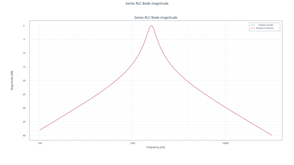
The magnitude diagram reaches a maximum of 0 dB at resonance. The complex-division result overlaps the independent analytical reference.
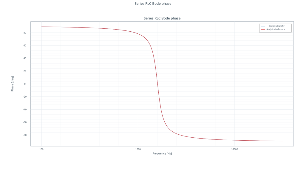
The phase diagram runs from approximately +90° to −90°, crossing zero at resonance. The two curves overlap.
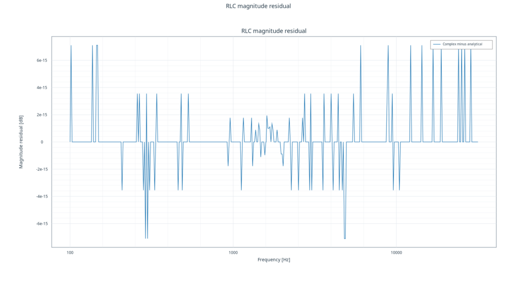
The gain residual is on the order of \(10^{-14}\,\mathrm{dB}\): this is double-precision numerical rounding, not experimental noise.
Interpreting the plots and their numerical precision
In the magnitude plot, the 0 dB maximum marks ideal resonance. Also examine the rise at low frequencies and the fall at high frequencies. In the phase plot, the zero crossing indicates that resistor output and input are in phase at resonance, with different phase signs on either side.
The residual plot compares two numerical representations of the same model, not theory with experimental measurements. A residual on the order of \(10^{-14}\,\mathrm{dB}\) is consistent with double-precision rounding; it does not establish fourteen-digit instrument accuracy or the absence of noise in a real experiment.
Procedure in the GX-TXT Octave Script Workspace
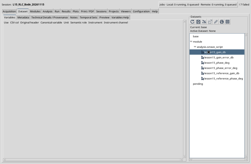
Create a new managed GX-TXT Session and import the three scripts, each with a distinct Script ID. Execute L15_00 and check that the two analytical Datasets have been published. Open L15_01 in the debugger, inspect the variables at the breakpoint, and continue until the intentional failure. Finally, run L15_02 and open the three native Plot Dataset graphs. To repeat the lesson from the beginning without ID collisions, create a new Session rather than deleting Dataset files outside the framework.
| Script | Expected outcome |
|---|---|
L15_00_Prepare_RLC_Reference.m |
2 analytical reference Datasets |
L15_01_Debug_Phase_Units.m |
Intentionally failed Job; no publication |
L15_02_RLC_Bode_Correct.m |
4 derived Datasets and 3 native GX-TXT plots |
Scientific interpretation and exercises
The peak at approximately 1.59 kHz is not a time-domain oscillation computed using ode45: it is a sinusoidal steady-state response in the frequency domain. Complementary information can be obtained by solving the circuit transient with differential equations, as introduced in Lesson 14. A smooth numerical curve cannot replace dimensional checks or scrutiny of the physical assumptions.
- Double \(R\) and predict how \(Q\), bandwidth, and peak height change. The ideal resonant frequency remains unchanged.
- Double \(C\) and calculate the expected new \(f_0\) analytically before changing the script.
- Use a sparser frequency grid. Explain why the sampled maximum may not coincide with \(f_0\) if the exact analytical frequency is not explicitly inserted.
- Calculate phase in radians and degrees at both cutoff frequencies.
- Change the output to the voltage across \(C\). Derive a new transfer function before publishing results; the resistor-output reference is no longer an appropriate scientific test.
Framework version and public references
Authoritative repository: GX-TXT on GitHub. Branch: maintenance/dev112. Public contract commit: 9f79a30661d6a3fe4a05d723be66aabd06ef2ebe (November 16, 2026). Published patch: DEV112 Release 2 P011. The teaching examples use the public contracts available at this commit:
The Octave scripts use the GPL-3.0-or-later license. All code comments and internal source documentation are in English.
Verified execution compatibility: the three scripts, publication of six Datasets, and rendering of three plots were tested with GX-TXT DEV112 R2 + P008. The P011 commit cited above identifies the most recent GitHub public contracts checked for this article; it does not imply that P011 itself was tested in execution.
Complete GNU Octave scripts
Expand each section to consult and copy the complete source code.
Script 00 — L15_00_Prepare_RLC_Reference.m
% Lesson 15 - Publish analytical reference data for a series RLC band-pass circuit.
% Course: GNU Octave with GX-TXT | public API reference DEV112 R2 P011
% Tested GX-TXT runtime: DEV112 R2 P008
% Pinned GitHub source: 9f79a30661d6a3fe4a05d723be66aabd06ef2ebe
% SPDX-License-Identifier: GPL-3.0-or-later
%
% Run once in a new managed GX-TXT Session.
% This script publishes deterministic analytical references, not measurements.

dataset_api = 'CANONICAL_DATASET_API_v2';
publication_api = 'DATASET_PUBLICATION_API_v2';
gxtxt_api_require({dataset_api, publication_api});
required = {dataset_api, 'list'; dataset_api, 'read_range'; ...
            publication_api, 'publish_series_batch'};
for k = 1:rows(required)
  if !gxtxt_api_has_operation(required{k,1}, required{k,2})
    error('Missing public GX-TXT operation: %s/%s.', ...
          required{k,1}, required{k,2});
  endif
endfor

% A series RLC circuit, driven by a 1 V sinusoidal input.
% The observed output voltage is the voltage across the resistance.
resistance_ohm = 20;
inductance_h = 10e-3;
capacitance_f = 1e-6;
f0_hz = 1 / (2*pi*sqrt(inductance_h*capacitance_f));
quality_factor = sqrt(inductance_h/capacitance_f) / resistance_ohm;
bandwidth_hz = resistance_ohm / (2*pi*inductance_h);

% Include the exact resonance frequency in the logarithmic sampling grid.
frequency_hz = sort([logspace(2, 4.5, 401)'; f0_hz]);
n = numel(frequency_hz);
assert(n == 402 && all(diff(frequency_hz) > 0));
omega = 2*pi*frequency_hz;

% Analytically evaluate |H| and angle(H) without a complex quotient.
% H(j*w) = R / (R + j*(w*L - 1/(w*C))).
reactance_ohm = omega*inductance_h - 1./(omega*capacitance_f);
gain_reference_db = 20*log10(resistance_ohm ./ ...
  sqrt(resistance_ohm^2 + reactance_ohm.^2));
phase_reference_deg = -atan2(reactance_ohm, resistance_ohm)*180/pi;
assert(all(isfinite(gain_reference_db)) && all(isfinite(phase_reference_deg)));
[~, resonance_row] = min(abs(frequency_hz-f0_hz));
assert(abs(gain_reference_db(resonance_row)) < 1e-11);
assert(abs(phase_reference_deg(resonance_row)) < 1e-11);

dataset_ids = {'lesson15_reference_gain_db', 'lesson15_reference_phase_deg'};
existing_ids = gxtxt_api_call(dataset_api, 'list', {});
for k = 1:numel(dataset_ids)
  if any(strcmp(existing_ids, dataset_ids{k}))
    error('Reference Dataset already exists: %s. Use a new Session.', ...
          dataset_ids{k});
  endif
endfor

frequency_variable = struct('variable_id','frequency_hz', ...
  'name','frequency_hz', 'display_label','Frequency', 'unit','Hz', ...
  'dtype','float64', 'value_kind','number','semantic_source','generator');
gain_variable = struct('variable_id','gain_db', ...
  'name','gain_db','display_label','Magnitude', 'unit','dB', ...
  'dtype','float64','value_kind','number','semantic_source','generator');
phase_variable = struct('variable_id','phase_deg', ...
  'name','phase_deg','display_label','Phase', 'unit','deg', ...
  'dtype','float64','value_kind','number','semantic_source','generator');

values = {gain_reference_db, phase_reference_deg};
definitions = {gain_variable, phase_variable};
descriptions = {'Analytical magnitude of resistor output, in dB', ...
                'Analytical phase of resistor output, in degrees'};
series = cell(1, numel(dataset_ids));
for k = 1:numel(dataset_ids)
  metadata = struct();
  metadata.('rlc.synthetic') = true;
  metadata.('rlc.topology') = 'series_resistor_output';
  metadata.('rlc.resistance_ohm') = resistance_ohm;
  metadata.('rlc.inductance_h') = inductance_h;
  metadata.('rlc.capacitance_f') = capacitance_f;
  metadata.('rlc.resonance_hz') = f0_hz;
  metadata.('rlc.quality_factor') = quality_factor;
  metadata.('rlc.method') = 'closed_form_reference';
  series{k} = struct('dataset_id', dataset_ids{k}, ...
    'contract','table.generic','storage','auto', ...
    'x_values',frequency_hz,'y_values',values{k}, ...
    'x_variable',frequency_variable,'y_variable',definitions{k}, ...
    'source','GX-TXT GNU Octave Lesson 15', ...
    'producer_version','1.0.0', ...
    'provenance','Deterministic analytical series RLC model', ...
    'notes',descriptions{k},'structured_metadata',metadata);
endfor

receipt = gxtxt_api_call(publication_api, 'publish_series_batch', ...
  {struct('series',{series})});
if !receipt.atomic || receipt.output_count != 2
  error('Atomic publication did not confirm two reference Datasets.');
endif
for k = 1:numel(dataset_ids)
  saved = gxtxt_api_call(dataset_api,'read_range', ...
    {dataset_ids{k}, {'frequency_hz',definitions{k}.variable_id},0,n});
  assert(max(abs(saved.frequency_hz.values(:)-frequency_hz)) < 1e-9);
  actual = saved.(definitions{k}.variable_id).values(:);
  assert(max(abs(actual-values{k})) < 1e-9);
endfor

fprintf('PASS: 2 analytical RLC reference Datasets published.\n');
fprintf('R = %.3f Ohm; L = %.5f H; C = %.9f F.\n', ...
        resistance_ohm, inductance_h, capacitance_f);
fprintf('f0 = %.6f Hz; Q = %.6f; bandwidth = %.6f Hz.\n', ...
        f0_hz, quality_factor, bandwidth_hz);
Script 01 — L15_01_Debug_Phase_Units.m
% Lesson 15 - Debug a deliberate phase-unit error in a complex RLC transfer.
% Course: GNU Octave with GX-TXT | public API reference DEV112 R2 P011
% Tested GX-TXT runtime: DEV112 R2 P008
% Pinned GitHub source: 9f79a30661d6a3fe4a05d723be66aabd06ef2ebe
% SPDX-License-Identifier: GPL-3.0-or-later
%
% Run after L15_00. Add a native debugger breakpoint at BREAKPOINT below.
% This Job is expected to fail; it creates no Dataset and no Plot Dataset.

dataset_api = 'CANONICAL_DATASET_API_v2';
gxtxt_api_require({dataset_api});
if !gxtxt_api_has_operation(dataset_api,'read_range')
  error('Missing public GX-TXT operation: read_range.');
endif

reference = gxtxt_api_call(dataset_api,'read_range', ...
  {'lesson15_reference_phase_deg',{'frequency_hz','phase_deg'},0,402});
frequency_hz = reference.frequency_hz.values(:);
expected_phase_deg = reference.phase_deg.values(:);
assert(numel(frequency_hz) == 402 && all(diff(frequency_hz)>0));

resistance_ohm = 20;
inductance_h = 10e-3;
capacitance_f = 1e-6;
omega = 2*pi*frequency_hz;
impedance_ohm = resistance_ohm + ...
  1i*(omega*inductance_h - 1./(omega*capacitance_f));
transfer = resistance_ohm ./ impedance_ohm;

% INTENTIONAL ERROR: angle() returns radians, not degrees.
% A phase plotted with a "degrees" label would be scientifically misleading.
phase_deg_wrong = angle(transfer);
maximum_phase_error_deg = max(abs(phase_deg_wrong - expected_phase_deg));
[~,high_frequency_row] = max(frequency_hz);

% BREAKPOINT: inspect phase_deg_wrong, expected_phase_deg,
% high_frequency_row, and maximum_phase_error_deg.
fprintf('At %.1f Hz: wrong phase = %.5f (radians).\n', ...
  frequency_hz(high_frequency_row),phase_deg_wrong(high_frequency_row));
fprintf('Correct phase = %.5f degrees; mismatch = %.5f.\n', ...
  expected_phase_deg(high_frequency_row),maximum_phase_error_deg);

% The expected FAILED Job prevents silent use of incorrectly labelled data.
if maximum_phase_error_deg > 30
  error('GXTXT:Lesson15:PhaseUnits', ...
    'The phase is in radians, not degrees. Multiply by 180/pi.');
endif
error('Unexpected success: the intentional phase-unit error escaped.');
Script 02 — L15_02_RLC_Bode_Correct.m
% Lesson 15 - Complex RLC transfer, validation and GX-TXT Bode plots.
% Course: GNU Octave with GX-TXT | public API reference DEV112 R2 P011
% Tested GX-TXT runtime: DEV112 R2 P008
% Pinned GitHub source: 9f79a30661d6a3fe4a05d723be66aabd06ef2ebe
% SPDX-License-Identifier: GPL-3.0-or-later
%
% Run in a managed GX-TXT Session after L15_00.
% Native Octave computes complex impedances; all GX-TXT Session, Dataset and
% Plot operations use documented public APIs through the Script Bridge.

dataset_api = 'CANONICAL_DATASET_API_v2';
publication_api = 'DATASET_PUBLICATION_API_v2';
plot_api = 'PLOT_DATASET_API_v4';
gxtxt_api_require({dataset_api, publication_api, plot_api});
required = {
  dataset_api,'list'; dataset_api,'read_range';
  publication_api,'publish_series_batch';
  plot_api,'new_spec'; plot_api,'validate_spec';
  plot_api,'upsert_plot'; plot_api,'render'; plot_api,'artifacts'
};
for k=1:rows(required)
  if !gxtxt_api_has_operation(required{k,1},required{k,2})
    error('Missing public GX-TXT operation: %s/%s.', ...
      required{k,1},required{k,2});
  endif
endfor

% Step 1: read the immutable analytical references by Dataset and Variable ID.
source_ids = {'lesson15_reference_gain_db','lesson15_reference_phase_deg'};
existing_ids = gxtxt_api_call(dataset_api,'list',{});
for k=1:numel(source_ids)
  if !any(strcmp(existing_ids,source_ids{k}))
    error('Missing reference Dataset %s. Run L15_00 first.',source_ids{k});
  endif
endfor
ref_gain = gxtxt_api_call(dataset_api,'read_range', ...
  {source_ids{1},{'frequency_hz','gain_db'},0,402});
ref_phase = gxtxt_api_call(dataset_api,'read_range', ...
  {source_ids{2},{'frequency_hz','phase_deg'},0,402});
frequency_hz = ref_gain.frequency_hz.values(:);
reference_gain_db = ref_gain.gain_db.values(:);
reference_phase_deg = ref_phase.phase_deg.values(:);
n = numel(frequency_hz);
if n != 402 || any(diff(frequency_hz)<=0) || ...
  max(abs(frequency_hz-ref_phase.frequency_hz.values(:)))>1e-9
  error('Reference frequency grids are missing or incompatible.');
endif

% Step 2: write the impedance equations with complex-valued Octave arrays.
resistance_ohm = 20;
inductance_h = 10e-3;
capacitance_f = 1e-6;
omega = 2*pi*frequency_hz;
z_resistor = resistance_ohm;
z_inductor = 1i*omega*inductance_h;
z_capacitor = 1./(1i*omega*capacitance_f);
z_total = z_resistor + z_inductor + z_capacitor;
transfer = z_resistor ./ z_total;
gain_linear = abs(transfer);
gain_db = 20*log10(gain_linear);
phase_deg = unwrap(angle(transfer))*180/pi;

% Step 3: independent physical and mathematical consistency checks.
f0_hz = 1/(2*pi*sqrt(inductance_h*capacitance_f));
quality_factor = sqrt(inductance_h/capacitance_f)/resistance_ohm;
bandwidth_hz = resistance_ohm/(2*pi*inductance_h);
omega_low = (-resistance_ohm + ...
  sqrt(resistance_ohm^2+4*inductance_h/capacitance_f)) / (2*inductance_h);
omega_high = (resistance_ohm + ...
  sqrt(resistance_ohm^2+4*inductance_h/capacitance_f)) / (2*inductance_h);
f_low = omega_low/(2*pi);
f_high = omega_high/(2*pi);
assert(abs((f_high-f_low)-bandwidth_hz)<1e-9);
assert(abs(sqrt(f_low*f_high)-f0_hz)<1e-9);

[~,resonance_row] = min(abs(frequency_hz-f0_hz));
if abs(frequency_hz(resonance_row)-f0_hz)>1e-9 || ...
   abs(gain_db(resonance_row))>1e-10 || ...
   abs(phase_deg(resonance_row))>1e-9
  error('At resonance the resistor output must be 0 dB and 0 degrees.');
endif
if any(gain_db>1e-8) || any(!isfinite(gain_db)) || ...
   any(!isfinite(phase_deg)) || ...
   phase_deg(1)<0 || phase_deg(end)>0
  error('Passive RLC magnitude or phase is unphysical.');
endif

gain_error_db = gain_db-reference_gain_db;
phase_error_deg = phase_deg-reference_phase_deg;
max_gain_error_db = max(abs(gain_error_db));
max_phase_error_deg = max(abs(phase_error_deg));
if max_gain_error_db>1e-8 || max_phase_error_deg>1e-7
  error('Complex impedance response disagrees with the analytical reference.');
endif
fprintf('R=%.1f Ohm, L=%.5f H, C=%.9f F.\n', ...
  resistance_ohm,inductance_h,capacitance_f);
fprintf('f0=%.6f Hz, Q=%.6f, -3 dB points=%.4f and %.4f Hz.\n', ...
  f0_hz,quality_factor,f_low,f_high);
fprintf('Max error: gain %.3g dB, phase %.3g deg.\n', ...
  max_gain_error_db,max_phase_error_deg);

% Step 4: atomically publish all derived series with physical units.
derived_ids = {'lesson15_gain_db','lesson15_phase_deg', ...
               'lesson15_gain_error_db','lesson15_phase_error_deg'};
for k=1:numel(derived_ids)
  if any(strcmp(existing_ids,derived_ids{k}))
    error('Derived Dataset exists: %s. Use a new Session.',derived_ids{k});
  endif
endfor
frequency_variable = struct('variable_id','frequency_hz', ...
  'name','frequency_hz','display_label','Frequency','unit','Hz', ...
  'dtype','float64','value_kind','number','semantic_source','plugin');
gain_variable = struct('variable_id','gain_db', ...
  'name','gain_db','display_label','Magnitude','unit','dB', ...
  'dtype','float64','value_kind','number','semantic_source','plugin');
phase_variable = struct('variable_id','phase_deg', ...
  'name','phase_deg','display_label','Phase','unit','deg', ...
  'dtype','float64','value_kind','number','semantic_source','plugin');
gain_error_variable = struct('variable_id','gain_error_db', ...
  'name','gain_error_db','display_label','Magnitude residual','unit','dB', ...
  'dtype','float64','value_kind','number','semantic_source','plugin');
phase_error_variable = struct('variable_id','phase_error_deg', ...
  'name','phase_error_deg','display_label','Phase residual','unit','deg', ...
  'dtype','float64','value_kind','number','semantic_source','plugin');
values = {gain_db,phase_deg,gain_error_db,phase_error_deg};
variables = {gain_variable,phase_variable, ...
             gain_error_variable,phase_error_variable};
descriptions = {'Complex impedance transfer magnitude in dB', ...
  'Complex impedance transfer phase in degrees', ...
  'Magnitude difference from analytical closed-form reference', ...
  'Phase difference from analytical closed-form reference'};
series = cell(1,numel(derived_ids));
for k=1:numel(derived_ids)
  metadata = struct();
  metadata.('rlc.synthetic') = true;
  metadata.('rlc.topology') = 'series_resistor_output';
  metadata.('rlc.resistance_ohm') = resistance_ohm;
  metadata.('rlc.inductance_h') = inductance_h;
  metadata.('rlc.capacitance_f') = capacitance_f;
  metadata.('rlc.resonance_hz') = f0_hz;
  metadata.('rlc.quality_factor') = quality_factor;
  metadata.('rlc.method') = descriptions{k};
  series{k} = struct('dataset_id',derived_ids{k}, ...
    'contract','table.generic','storage','auto', ...
    'x_values',frequency_hz,'y_values',values{k}, ...
    'x_variable',frequency_variable,'y_variable',variables{k}, ...
    'source','GX-TXT GNU Octave Lesson 15','producer_version','1.0.0', ...
    'source_dataset_ids',{source_ids}, ...
    'provenance','GNU Octave complex RLC and public GX-TXT Dataset services', ...
    'notes',descriptions{k},'structured_metadata',metadata);
endfor
receipt = gxtxt_api_call(publication_api,'publish_series_batch', ...
  {struct('series',{series})});
if !receipt.atomic || receipt.output_count != numel(derived_ids)
  error('Atomic publication did not confirm four derived Datasets.');
endif

% Step 5: verify every stored Dataset through public read_range.
for k=1:numel(derived_ids)
  saved = gxtxt_api_call(dataset_api,'read_range', ...
    {derived_ids{k},{'frequency_hz',variables{k}.variable_id},0,n});
  actual = saved.(variables{k}.variable_id).values(:);
  if numel(actual)!=n || ...
     max(abs(saved.frequency_hz.values(:)-frequency_hz))>1e-9 || ...
     max(abs(actual-values{k}))>1e-8
    error('Read-back verification failed for %s.',derived_ids{k});
  endif
endfor

% Step 6: create native persistent plots with logarithmic frequency axes.
plot_definitions = {
  'lesson15_bode_gain','Series RLC Bode magnitude', ...
  {'Complex transfer','Analytical reference'}, ...
  {'lesson15_gain_db','lesson15_reference_gain_db'}, ...
  {'gain_db','gain_db'}, 'Magnitude [dB]';
  'lesson15_bode_phase','Series RLC Bode phase', ...
  {'Complex transfer','Analytical reference'}, ...
  {'lesson15_phase_deg','lesson15_reference_phase_deg'}, ...
  {'phase_deg','phase_deg'}, 'Phase [deg]';
  'lesson15_bode_gain_residual','RLC magnitude residual', ...
  {'Complex minus analytical'}, {'lesson15_gain_error_db'}, ...
  {'gain_error_db'}, 'Magnitude residual [dB]'
};
for p=1:rows(plot_definitions)
  plot_id = plot_definitions{p,1};
  title_text = plot_definitions{p,2};
  labels = plot_definitions{p,3};
  dataset_list = plot_definitions{p,4};
  variable_list = plot_definitions{p,5};
  ylabel_text = plot_definitions{p,6};
  spec = gxtxt_api_call(plot_api,'new_spec',{'plot.dataset.xy',title_text});
  panel = spec.panels{1};
  panel.id = ['bode_panel_',num2str(p)];
  panel.title = title_text;
  panel.axes = struct('x',struct('label','Frequency [Hz]','scale','log'), ...
    'y_left',struct('label',ylabel_text,'scale','linear'));
  curves=cell(1,numel(labels));
  for k=1:numel(labels)
    curves{k}=struct('id',['rlc_trace_',num2str(k)], ...
      'label',labels{k},'dataset_id',dataset_list{k}, ...
      'x_variable_id','frequency_hz', ...
      'y_variable_id',variable_list{k},'axis','left','kind','line');
  endfor
  panel.series=curves;
  spec.panels={panel};
  if !gxtxt_api_call(plot_api,'validate_spec',{spec})
    error('PlotSpec validation failed for %s.',plot_id);
  endif
  plot_ref=gxtxt_api_call(plot_api,'upsert_plot',{plot_id,spec});
  gxtxt_api_call(plot_api,'render',{plot_ref});
  artifacts=gxtxt_api_call(plot_api,'artifacts',{plot_ref});
  fprintf('Created native Plot Dataset %s.\n',plot_id);
  disp(artifacts);
endfor
fprintf('PASS: 4 derived canonical Datasets and 3 native Bode plots.\n');
fprintf('PASS: resonance, bandwidth, gain and phase validated.\n');
Other steps of this project
- Lesson 01 — Your First GNU Octave Script in GX-TXT
- Lesson 02 — Variables, Data Types and Operators in GNU Octave with GX-TXT
- Lesson 03 — Vectors and Matrices in GNU Octave with GX-TXT: Temperature Measurement Analysis
- Lesson 04 — Conditions, Loops, and Functions. Simulating Newton’s Law of Cooling
- Lesson 05: Scientific Datasets and Variable IDs
- Lesson 06 — Selecting and Reading Experimental Data with GNU Octave and GX-TXT