

Lesson 13 — Spectral Analysis: FFT, Sampling and Windows with GNU Octave and GX-TXT
From a Time-Domain Signal to Its Frequency Components
An electrical signal may look complex when viewed in the time domain, yet consist of the sum of just a few simple oscillations. This lesson teaches how to use the discrete Fourier transform, compute a one-sided amplitude spectrum, identify an error in the sampling frequency, and understand spectral leakage. The results will be saved as GX-TXT Datasets and displayed using persistent plots.
The experiment uses synthetic data only, so that we know precisely which frequencies and amplitudes we need to recover.
Reference version: GX-TXT 0.9.8.10-dev-112, Release 2, patch P008, GitHub release. Verified source commit: 17ff2a7f93de0612015a873e626f87dbeb56b6a2. Language: GNU Octave. The scripts are licensed under GPL-3.0-or-later and contain comments in English.
What We Will Learn
By the end of this lesson, we will be able to define a time vector in Octave, add sinusoids, calculate sampling frequency and spectral-bin spacing, read canonical Datasets through variable identifiers, apply numerical transformations through public APIs, work with complex numbers, and assess the reliability of a spectrum. We will also use the GX-TXT debugger to investigate an intentional error and publish the processed results without manipulating internal files.
Connection with the Previous Twelve Lessons
In Lessons 01–04, we learned syntax, numerical types, complex numbers, vectors, matrices, conditions, loops, and functions. Lessons 05–07 introduced Datasets, Variable IDs, canonical reading, and publication; Lesson 07 already generated sampled sinusoids using GNU Octave. Lesson 08 introduced persistent plots and debugging, which were revisited in Lessons 09–12 for statistics, regression, numerical calculus, and linear algebra.
What is new in Lesson 13 is not generating another sine wave: it is finding which oscillations make up a measurement, interpreting frequency information, and understanding the limitations of the results. We will reuse previously introduced concepts—vectors, Octave structures, cell arrays, Dataset IDs, Variable IDs, and persistent plots—without redefining them. Instead, we will study the FFT, discrete frequencies, normalization, windows, and reconstruction step by step.
| Previously acquired knowledge | How we use it here | New concept |
|---|---|---|
| Vectors, element-wise operations (03, 07) | Generate time-domain samples | Relationship between samples and frequencies |
| Complex numbers (02) | Reconstruct coefficients from real and imaginary parts | FFT magnitude, phase, and symmetry |
| Canonical Datasets (05–07) | Read time and voltage using Variable IDs | Validate the sampling interval |
| GX-TXT debugger (08–12) | Inspect an incorrect parameter | Physical error on the frequency axis |
| Publication and Plot Dataset (07–12) | Save spectra and plots | Frequency-domain Datasets |
The Experiment: Two Sinusoidal Components
The first signal is defined by
\[v(t)=0.20+1.25\,\sin(2\pi\cdot 50\,t+0.15)+0.50\,\sin(2\pi\cdot 120\,t-0.30)\]
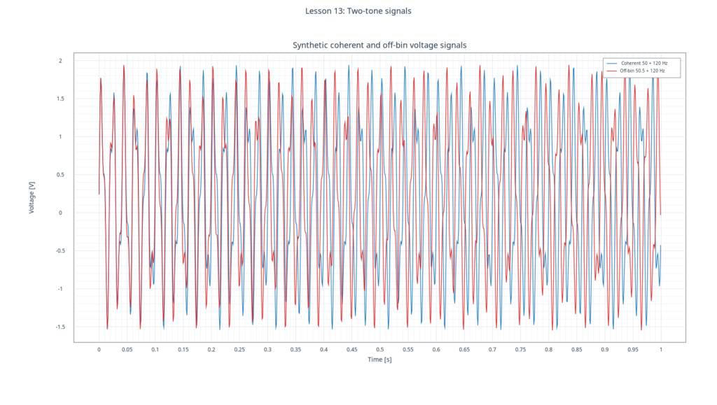
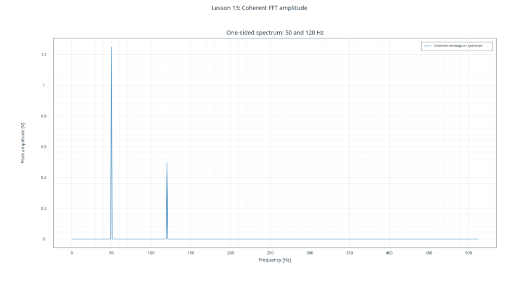
Voltage is expressed in volts and time in seconds. The signal contains a DC component of 0.20 V, a 50 Hz sine wave with a peak amplitude of 1.25 V, and a 120 Hz sine wave with a peak amplitude of 0.50 V. Phases are expressed in radians.
A second signal retains the amplitudes and the higher frequency, but replaces the first component with 50.5 Hz. This small change lets us observe what happens when a frequency does not coincide with an FFT bin.
Lesson 13 uses the following parameters:
| Quantity | Symbol | Value |
|---|---|---|
| Sampling frequency | \(f_s\) | 1024 Hz |
| Number of samples | \(N\) | 1024 |
| Sampling interval | \(\Delta t=\frac{1}{f_s}\) | 0.0009765625 s |
| Record duration | \(T=\frac{N}{f_s}\) | 1 s |
| Bin spacing | \(\Delta f=\frac{f_s}{N}\) | 1 Hz |
| Nyquist frequency | \(f_N=\frac{f_s}{2}\) | 512 Hz |
In Octave, we construct the time sequence as follows:
sample_rate_hz = 1024;
sample_count = 1024;
time_s = (0:sample_count - 1)' / sample_rate_hz;
The : operator generates a sequence, the apostrophe ' converts it into a column vector, and division by the sampling frequency converts the indices into seconds. The expression sin(2*pi*f*time_s + phase) evaluates the sine wave at every instant.
From Sample Index to Physical Time
In our experiment, the sample with mathematical index \(n\) is observed at time \(t_n=\frac{n}{f_s}\). For \(n=0,\ldots,1023\), we obtain 1024 samples, but the last timestamp is \(1023/1024=0.9990234375\) s. We must not add a sample at \(t=1\) s: this would repeat the initial point of the period, yielding 1025 values and changing the spectral grid.
The record duration used in the DFT is \(T=\frac{N}{f_s}=1\) s. It must not be confused with the difference between the first and last timestamps, which equals \(\frac{N-1}{f_s}\). This distinction makes the time-vector construction consistent with the FFT bins.
For the 50 Hz component, the record contains exactly 50 periods, and for the 120 Hz component it contains 120: both are coherent with the observed time window. The second signal, however, contains 50.5 periods of the lower-frequency component. This will be our controlled demonstration of spectral leakage.
From Time to Frequency: A Change of Representation
The horizontal axis of the first plot is time (s) and the vertical axis is voltage (V). After the DFT, the horizontal axis represents frequency (Hz). These are not new measurements: they are a different mathematical representation of the same sample sequence.
Bin \(k\), in the nonnegative half of the spectrum, corresponds to \(f_k=\frac{k f_s}{N}\). Here, bin spacing is 1 Hz. Bins 50 and 120 therefore correspond exactly to the two frequencies of the first signal. Zero represents the DC component; bin 512 is the Nyquist frequency.
What the FFT Computes
The discrete Fourier transform of \(N\) samples is
\[X[k]=\sum_{n=0}^{N-1}x[n] \,e^{-i\,2\pi kn/N},\qquad k=0,\ldots,N-1\]
In Octave, array indices start at 1, whereas the mathematical formula starts at 0. Consequently, when \(\Delta f=1\) Hz, the 50 Hz bin is stored at X(51), and the 120 Hz bin at X(121).
Complex Coefficients, Magnitude, and Phase
The DFT result is not directly a list of amplitudes in volts: each coefficient \(X[k]\) is a complex number. Its real and imaginary parts jointly carry information about both amplitude and phase. In Octave, the magnitude is obtained using abs(z), while the angle is obtained using angle(z) (radians). For example, the 50 Hz component is at array position 51 because Octave indices start at one.
For a real-valued sinusoid, \(X[N-k]\) is the complex conjugate of \(X[k]\) (when \(k\) is not an endpoint). The negative-frequency half therefore repeats the information in the positive-frequency half. This is why a one-sided spectrum is possible. However, retaining only the magnitude \(|X[k]|\) loses phase information: the original signal cannot be reconstructed uniquely from amplitudes alone.
A practical example: two sinusoids with the same amplitude and frequency but different phases produce peaks of equal amplitude; their complex coefficients, however, are different.
For real-valued signals, FFT coefficients are complex and exhibit conjugate symmetry. A one-sided spectrum retains only nonnegative frequencies. With the standard FFT normalization (backward, meaning an unscaled forward transform), the correct peak amplitude of a bin-coherent tone at an interior bin is
\[A_k=\frac{2|X[k]|}{N\,G_c}\]
where \(G_c\) is the coherent gain of the window. The factor of 2 must not be applied to the DC component or to the Nyquist bin, when present.
Why We Normalize the Spectrum
With normalization = backward, the forward transform is not divided by \(N\); scaling of the inverse is handled by the inverse transform. To obtain a physical amplitude, we must therefore divide the FFT magnitude by \(N\) and correct for the window coherent gain \(G_c\).
Interior bins in the one-sided spectrum must also be multiplied by two: for a real-valued signal, the sinusoidal component is shared between two symmetric frequencies. The DC and Nyquist bins must not be doubled. The public oneSided operation handles this scaling; the script then divides the magnitude by \(N\,G_c\).
For a rectangular window, \(G_c=1\), and for tones exactly centered on bins we recover peak amplitudes of 1.25 V and 0.50 V—peak values, not RMS. To convert individual sinusoidal peak amplitudes to RMS, divide by \(\sqrt{2}\): approximately 0.884 V and 0.354 V. The RMS value of the complete signal, on the other hand, requires accounting for all components and any DC offset.
Power spectral density (PSD) is a different quantity, with a different normalization and typical units of \(\mathrm{V}^2/\mathrm{Hz}\); it is used to study how power or noise is distributed across frequencies. A graph in peak volts is not a PSD merely because its horizontal axis is frequency.
Note: an amplitude spectrum is not a power spectral density (PSD). We will not call the result of this exercise a PSD.
The Workflow Through the Scripts
Preparation – L13_00_Prepare_Two_Tone_Signals.m
The first script generates the two signals, publishes two canonical Datasets, and reads them back through the public APIs to verify that storage preserved the samples. Publication is an atomic transaction.
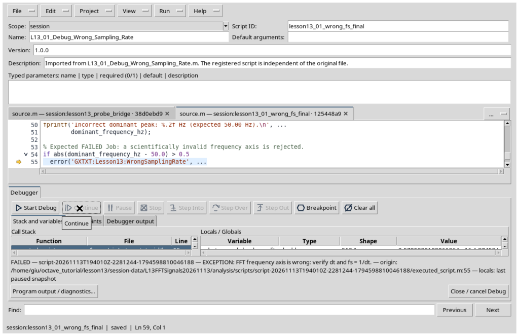
Debugger – L13_01_Debug_Wrong_Sampling_Rate.m
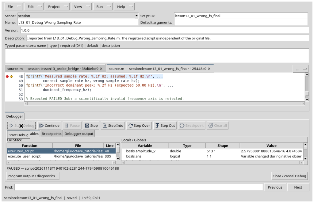
The second script contains an intentional scientific error: it uses \(f_s=512\) Hz to construct the frequency axis, even though the time vector establishes that \(f_s=1024\) Hz. The FFT coefficient amplitudes remain unchanged, but the reported frequency of the main peak becomes 25 Hz instead of 50 Hz.
In the GX-TXT Octave Script Workspace, import the file under a distinct identifier and select Run → Debug Session script. Set a breakpoint near the BREAKPOINT comment, then inspect correct_sample_rate_hz, wrong_sample_rate_hz, measured_step_s, and dominant_frequency_hz. After selecting Continue, the Job must end with the expected instructional error: this is not a framework bug, but the correct detection of a false assumption.
This example does not simulate the physical phenomenon of aliasing: it changes only the sampling frequency used to label the bins. Aliasing instead occurs when the signal is actually sampled at an insufficient rate.
Understanding the Error Before Correcting It
In the intentionally incorrect run, the sample vector remains unchanged and the FFT produces the same coefficients. Only the value passed to frequencyGrid changes: using \(f_s=512\) Hz rather than 1024 Hz makes the bin spacing \(0.5\) Hz. As a result, bin \(k=50\), which should be labeled 50 Hz, is shown at 25 Hz.
The debugger lets us compare the time step actually read from the Dataset, the sampling rate inferred from that step, and the frequency entered incorrectly. The check that triggers the intentional failure is a scientific consistency check, not a malfunction of the FFT algorithm.
It is essential to distinguish this error from aliasing: aliasing occurs during actual sampling, when frequencies that are too high cannot be distinguished at the chosen sampling rate \(f_s\). With \(f_s=1024\) Hz, for example, a 700 Hz component can fold back to 324 Hz: \(1024-700=324\). The 25 Hz value shown in this lesson is not an alias.
Correct Analysis – L13_02_FFT_Spectrum_Correct.m
The third script derives the sampling frequency directly from the Dataset timestamps, checks the uniformity of the intervals, removes the mean, computes the FFT and the frequency axis through GX-TXT services, selects the one-sided coefficients, and recovers physical amplitudes. It also compares a rectangular window with a periodic Hann window for the 50.5 Hz signal and checks the inverse FFT.
Finally, it creates four derived Datasets and three persistent GX-TXT plots: time-domain signals, coherent-frequency spectrum, and window comparison.
The GX-TXT Public APIs Used
The following operations are specified in the public contracts of the stated version. In this lesson, they are not simply names to copy: they connect the Octave code to the scientific infrastructure.
| API / operation | Purpose and educational meaning |
|---|---|
gxtxt_api_require, gxtxt_api_has_operation | Check that the Session exposes the required contracts and operations before calculation |
gxtxt_api_call(api, operation, args) | Invokes a public service, passing its arguments as an Octave cell array |
CANONICAL_DATASET_API_v2 / list | Lists stable identifiers of published Datasets |
CANONICAL_DATASET_API_v2 / read_range | Reads samples from known variables using Dataset ID, Variable ID, offset, and row count |
NUMERIC_API_v1 / detrend | Removes a mean or a trend without implicitly changing the sampling timestamps |
NUMERIC_API_v1 / window | Generates window weights and provides coherent gain for amplitude correction |
NUMERIC_API_v1 / fft | Computes the transform without hidden scientific scaling; returns real and imaginary parts |
NUMERIC_API_v1 / frequencyGrid | Calculates frequencies, \(\Delta f\), and Nyquist from \(f_s\) and \(N\) |
NUMERIC_API_v1 / oneSided | Selects nonnegative frequencies and, with scaling=amplitude, doubles interior bins only |
NUMERIC_API_v1 / ifft | Computes the inverse, useful for checking that the transformation preserves the data |
DATASET_PUBLICATION_API_v2 / publish_series_batch | Publishes scientific series, metadata, and provenance together |
PLOT_DATASET_API_v4 | Creates, validates, registers, renders, and exposes plots that reference canonical Datasets |
The New Numerical Operations, Call by Call
Previous lessons have already explained how to check dependencies and invoke a service with gxtxt_api_call. Here we focus on the numerical contracts introduced for the first time. In every example, the third argument of gxtxt_api_call is an Octave cell array containing the operation arguments in the order specified by the contract.
| Public operation | Arguments used in the script | Result used | Why it is needed |
|---|---|---|---|
| detrend | voltage vector; structure with method = mean | values | Removes the mean before spectral analysis |
| window | rectangular or hann name; N; structure with sampling = periodic | values; coherent_gain | Provides weights and the amplitude-correction factor |
| fft | vector; structure with nfft = N and normalization = backward | real; imaginary | Computes the complex DFT coefficients |
| frequencyGrid | sampling frequency; N; structure with representation = one_sided | frequencies; df and other grid information | Associates physical units with bins |
| oneSided | real; imaginary; structure with scaling = amplitude and nfft = N | real; imaginary | Selects the nonnegative half and handles interior bins correctly |
| ifft | real and imaginary parts; structure with nfft = N and normalization = backward | real; imaginary | Reconstructs the signal to check the transform |
Checks before the FFT. The script compares the time axes of the two Datasets; computes the intervals with the native Octave function diff; estimates the step with median; checks that the intervals are positive and uniform; and finally uses \(f_s=\frac{1}{\Delta t}\). This prevents an analysis parameter from being mistaken for a directly observed property.
Response checks. Values must have consistent lengths; frequencies and amplitudes must refer to the same bins; and the real and imaginary parts must be combined in the same order. complex(re, im) is a native Octave function, whereas fft called through NUMERIC_API_v1 is a GX-TXT public service.
Errors to prevent. Do not confuse a Dataset ID with a file, change the order of arguments in the cell array, call frequencyGrid with an assumed sampling frequency, multiply by two again after conversion by oneSided, or divide by \(N\) twice.
Three Calls to Examine in the Code
Consider three operations introduced in this lesson. The first argument identifies the public service, the second names the operation, and the third holds its parameters in an Octave cell array.
centered = gxtxt_api_call('NUMERIC_API_v1', 'detrend', ...
  {voltage_values, struct('method', 'mean')});

grid = gxtxt_api_call('NUMERIC_API_v1', 'frequencyGrid', ...
  {1024, 1024, struct('representation', 'one_sided')});

hann_window = gxtxt_api_call('NUMERIC_API_v1', 'window', ...
  {'hann', 1024, struct('sampling', 'periodic')});
In the first call, voltage_values represents the data vector, while centered.values contains the mean-removed values. In the second, we request the frequency grid by explicitly providing the sampling frequency and sample count, both of which are essential for interpreting the horizontal axis. In the third, we request 1024 weights for the periodic Hann window and its coherent_gain, which we use to express amplitudes in the original physical units.
None of these three calls reads internal GX-TXT files: the data come from canonical APIs, and processing is performed through the public numerical-service contract.
For example, the call
fft_result = gxtxt_api_call('NUMERIC_API_v1', 'fft', ...
  {voltage_values, struct('nfft', 1024, 'normalization', 'backward')});
complex_bins = complex(fft_result.real, fft_result.imaginary);
shows that gxtxt_api_call does not directly accept a variable-length list of Octave arguments: its final parameter is a cell array. The service returns separate real and imaginary parts; using complex, we reconstruct the complex coefficients to calculate abs.
The frequencyGrid function cannot automatically infer \(f_s\) from the FFT array alone: sampling frequency comes from the acquisition process. That is why we derive and validate it from the time-domain Dataset.
Windowing: Why Change the Sample Weights?
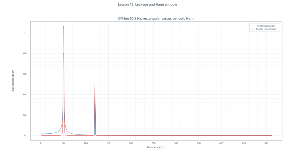
The DFT interprets the \(N\) samples as one period of a sequence repeated indefinitely. If the signal contains an integer number of periods within the record, its endpoints join periodically and the tone is concentrated in one bin. If the sine wave contains 50.5 periods, the periodic junction has a discontinuity: its energy spreads across many bins. This is spectral leakage.
The rectangular window assigns a weight of 1 to each sample. The periodic Hann window instead uses, for \(n=0,\ldots,N-1\),
\[w[n]=\frac{1}{2}-\frac{1}{2}\cos\!\left(\frac{2\pi n}{N}\right)\]
Samples near the endpoints are attenuated, reducing the discontinuity at the periodic junction. This produces lower sidelobes but a wider main lobe: it is not a cost-free transformation. The periodic Hann window has coherent gain \(G_c=0.5\); the rectangular window has a gain of 1.
Coherent gain and scalloping loss are not the same thing. Correction by \(G_c\) restores the amplitude of a bin-aligned tone after windowing. If the tone falls between bins, the maximum may still be lower than the true value after that correction: this is scalloping loss. Therefore, the largest single bin should not automatically be treated as an exact measurement of a noncoherent tone.
Another trade-off concerns identifying two nearby frequencies. The width of the main lobe can make two tones appear less distinctly separated, whereas sidelobe suppression can reveal a weak component next to a strong one. Window selection depends on the purpose of the analysis.
Windowing and Spectral Leakage
The 50.5 Hz signal does not contain an integer number of cycles in the observed second; with a rectangular window, energy spreads across multiple bins. A periodic Hann window reduces sidelobes but broadens the main lobe. Its coherent gain, here 0.5, must be included when scaling amplitudes.
The Hann window does not make the amplitude of a tone between bins perfectly accurate: misalignment still causes a loss known as scalloping loss. The height of an isolated maximum should not be interpreted as an exact estimate in every situation.
In our numerical verification, for this synthetic example only and at the 70 Hz bin, the amplitude associated with leakage decreases from approximately \(0.0170\) V (rectangular) to \(0.0000536\) V (Hann). This comparison concerns that specific bin; it is not a promise of uniform reduction throughout the entire spectrum.
Spectral Resolution, Duration, and Zero-Padding
Bin spacing is \(\Delta f=\frac{f_s}{N}=\frac{1}{T}\). If we keep \(f_s=1024\) Hz and observe the signal for 2 s, we use 2048 samples and obtain \(\Delta f=0.5\) Hz. The observation duration changes; the Nyquist frequency, however, remains \(512\) Hz because it depends on \(f_s\).
Increasing nfft beyond the number of samples by padding the signal with zeros (zero-padding) produces a finer frequency grid but does not add time-domain information. It may help visualize and interpolate peaks; it does not have the same effect as doubling the measurement duration. In this script, we use \(\mathrm{nfft}=N=1024\), so the relationship between sampling, duration, and frequency grid remains transparent.
Inverse FFT
Using ifft, we reconstruct the mean-removed signal and then restore the DC component. The maximum difference between the original and reconstructed samples should be close to machine numerical precision. This check verifies coefficient consistency and ordering; it does not, by itself, prove that our physical interpretation of the spectrum is correct.
How We Evaluate the Reconstruction
For the coherent signal, the script removes the mean before computing the FFT, passes the full set of complex coefficients—not just the positive-frequency half—to the IFFT, and adds the mean back to the reconstructed vector. The test computes the maximum absolute sample-by-sample difference.
A very small error confirms that the two transforms are consistent within the available numerical precision. It does not, on its own, establish that the original sampling satisfied Nyquist or that the spectrum accurately describes a real physical system: the IFFT can reconstruct an improperly sampled sequence as well.
Expected Numerical Results
| Check | Expected result |
|---|---|
| Main frequency | 50.000 Hz |
| Second frequency | 120.000 Hz |
| Main amplitude | 1.250 V peak |
| Second amplitude | 0.500 V peak |
| Bin spacing | 1 Hz |
| Nyquist | 512 Hz |
| Periodic Hann coherent gain | 0.5 |
| Input / derived Datasets | 2 / 4 |
| Persistent plots | 3 |
These values provide a reference for checking the results of your own run, distinguishing numerical correctness from the physical interpretation of the spectrum.

How to Reproduce the Lesson
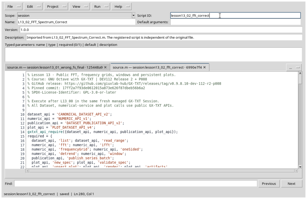
Create a new independent Session in GX-TXT, open Viewers → Octave Scripts, import L13_00, assign a distinct Script ID, and save it. Run the script using Run → Open Script Runner and verify that it completes. Open L13_01 under a second Script ID and inspect the intentional error in the debugger. Finally, import and run L13_02 under a third Script ID; check the Datasets and plots in the main window.
The scripts publish canonical identifiers in create-only mode. To repeat the complete experiment, start a new Session rather than deleting or modifying internal registration files.
What Makes This Experiment Reproducible
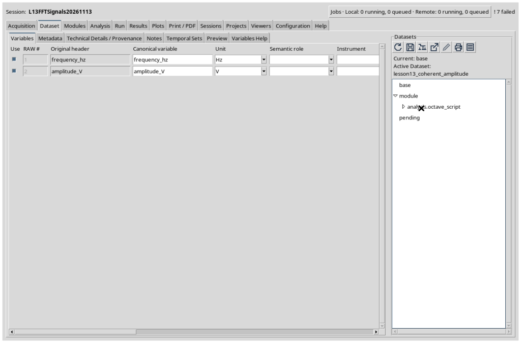
The workflow to verify is: define the synthetic signal and its sampling frequency; publish the two Datasets with physical units; read them canonically without accessing internal files; check time intervals; perform numerical analysis through public APIs; publish the four derived Datasets; and register the three persistent plots.
Comparing predicted and observed values distinguishes the correctness of mathematical operations from the interpretation of a measurement. A frequency shown on the X axis is meaningful only if derived from the actual time step; an amplitude expressed in volts requires normalization consistent with the chosen convention.
Exercises
- Change the amplitude of the 120 Hz component and predict how the corresponding bin will change.
- Increase \(N\) while keeping \(f_s\) unchanged. What happens to duration and bin spacing?
- Compare a rectangular window and a Hann window at a noncoherent frequency; explain why the main-lobe width changes.
- Add a 700 Hz component actually sampled at 1024 Hz, and predict the alias frequency \(1024-700=324\) Hz. Distinguish this effect from the intentional error in the second script.
References to Public Source Code
- Octave Script Bridge API v1
- Canonical Dataset API v2
- Dataset Publication API v2
- Numeric API v1
- Plot Dataset API v4
The complete scripts, with comments in English, are available in the expandable sections at the end of the article and in the downloadable course materials.
Complete GNU Octave Scripts
Open the expandable sections to inspect or copy the three scripts. Code comments are in English.
L13_00_Prepare_Two_Tone_Signals.m
% Lesson 13 - Publish synthetic signals for the Fourier transform.
% Course: GNU Octave with GX-TXT | DEV112 Release 2 + P008
% GitHub commit: 17ff2a7f93de0612015a873e626f87dbeb56b6a2
% SPDX-License-Identifier: GPL-3.0-or-later
%
% Execute once in a new managed GX-TXT Session.
% The two traces are deterministic synthetic examples, not measurements.

dataset_api = 'CANONICAL_DATASET_API_v2';
publication_api = 'DATASET_PUBLICATION_API_v2';
gxtxt_api_require({dataset_api, publication_api});
assert(gxtxt_api_has_operation(dataset_api, 'list'));
assert(gxtxt_api_has_operation(dataset_api, 'read_range'));
assert(gxtxt_api_has_operation(publication_api, 'publish_series_batch'));

sample_rate_hz = 1024;
sample_count = 1024;
time_s = (0:sample_count - 1)' / sample_rate_hz;
fundamental_amplitude_v = 1.25;
second_amplitude_v = 0.50;
offset_v = 0.20;

% Integer-cycle tones occupy exactly one FFT bin per component.
coherent_v = offset_v + ...
  fundamental_amplitude_v * sin(2*pi*50*time_s + 0.15) + ...
  second_amplitude_v * sin(2*pi*120*time_s - 0.30);

% A half-bin frequency demonstrates spectral leakage without random noise.
offbin_v = offset_v + ...
  fundamental_amplitude_v * sin(2*pi*50.5*time_s + 0.15) + ...
  second_amplitude_v * sin(2*pi*120*time_s - 0.30);
assert(numel(time_s) == sample_count);
assert(all(isfinite(coherent_v)) && all(isfinite(offbin_v)));

ids = {'lesson13_signal_coherent', 'lesson13_signal_offbin'};
existing = gxtxt_api_call(dataset_api, 'list', {});
for k = 1:numel(ids)
  if any(strcmp(existing, ids{k}))
    error('Source Dataset already exists: %s. Use a fresh Session.', ids{k});
  endif
endfor

time_var = struct('variable_id', 'time_s', ...
  'name', 'time_s', 'display_label', 'Elapsed time', ...
  'unit', 's', 'dtype', 'float64', 'value_kind', 'number', ...
  'semantic_source', 'generator');
voltage_var = struct('variable_id', 'voltage_V', ...
  'name', 'voltage_V', 'display_label', 'Synthetic voltage', ...
  'unit', 'V', 'dtype', 'float64', 'value_kind', 'number', ...
  'semantic_source', 'generator');

all_values = {coherent_v, offbin_v};
all_labels = {'Two coherent sinusoids at 50 and 120 Hz', ...
              'Half-bin tone at 50.5 Hz plus coherent 120 Hz'};
series = cell(1, 2);
for k = 1:2
  metadata = struct();
  metadata.('simulation.synthetic') = true;
  metadata.('simulation.sample_rate_hz') = sample_rate_hz;
  metadata.('simulation.sample_count') = sample_count;
  metadata.('simulation.offset_v') = offset_v;
  metadata.('simulation.description') = all_labels{k};
  series{k} = struct('dataset_id', ids{k}, 'contract', 'table.generic', ...
    'storage', 'auto', 'x_values', time_s, 'y_values', all_values{k}, ...
    'x_variable', time_var, 'y_variable', voltage_var, ...
    'producer_version', '1.0.0', ...
    'source', 'GX-TXT GNU Octave Lesson 13', ...
    'provenance', 'Deterministic simulated two-tone voltage records', ...
    'notes', all_labels{k}, 'structured_metadata', metadata);
endfor

receipt = gxtxt_api_call(publication_api, 'publish_series_batch', ...
  {struct('series', {series})});
if !receipt.atomic || receipt.output_count != 2
  error('Atomic publication failed to confirm two source Datasets.');
endif

% Read back through the canonical public Dataset API, not the storage files.
for k = 1:2
  result = gxtxt_api_call(dataset_api, 'read_range', ...
    {ids{k}, {'time_s', 'voltage_V'}, 0, sample_count});
  assert(numel(result.time_s.values) == sample_count);
  assert(max(abs(result.time_s.values(:) - time_s)) < 1e-12);
  assert(max(abs(result.voltage_V.values(:) - all_values{k})) < 1e-10);
endfor

fprintf('PASS: 2 canonical synthetic source Datasets published.\n');
fprintf('Sampling: fs=%g Hz, N=%d, duration=%.3f s, df=%.3f Hz.\n', ...
        sample_rate_hz, sample_count, ...
        sample_count/sample_rate_hz, sample_rate_hz/sample_count);
L13_01_Debug_Wrong_Sampling_Rate.m
% Lesson 13 - An intentional sampling-frequency error for the debugger.
% Course: GNU Octave with GX-TXT | DEV112 Release 2 + P008
% GitHub commit: 17ff2a7f93de0612015a873e626f87dbeb56b6a2
% SPDX-License-Identifier: GPL-3.0-or-later
%
% Run after L13_00. Set a breakpoint at the marked line.
% This program MUST fail its scientific frequency validation.
% It publishes no Dataset and creates no plot.

dataset_api = 'CANONICAL_DATASET_API_v2';
numeric_api = 'NUMERIC_API_v1';
gxtxt_api_require({dataset_api, numeric_api});
assert(gxtxt_api_has_operation(dataset_api, 'read_range'));
assert(gxtxt_api_has_operation(numeric_api, 'fft'));
assert(gxtxt_api_has_operation(numeric_api, 'frequencyGrid'));
assert(gxtxt_api_has_operation(numeric_api, 'oneSided'));

n = 1024;
data = gxtxt_api_call(dataset_api, 'read_range', ...
  {'lesson13_signal_coherent', {'time_s', 'voltage_V'}, 0, n});
t = data.time_s.values(:);
v = data.voltage_V.values(:);
if numel(t) != n || numel(v) != n || any(diff(t) <= 0)
  error('Missing or invalid source record: run L13_00 first.');
endif

measured_step_s = median(diff(t));
correct_sample_rate_hz = 1 / measured_step_s;

% INTENTIONAL ERROR: the assumed sample rate is half the true value.
% Fourier coefficients remain unchanged, but every displayed Hz value halves.
wrong_sample_rate_hz = 512;
raw_fft = gxtxt_api_call(numeric_api, 'fft', ...
  {v - mean(v), struct('nfft', n, 'normalization', 'backward')});
wrong_grid = gxtxt_api_call(numeric_api, 'frequencyGrid', ...
  {wrong_sample_rate_hz, n, struct('representation', 'one_sided')});
positive = gxtxt_api_call(numeric_api, 'oneSided', ...
  {raw_fft.real, raw_fft.imaginary, struct('scaling', 'amplitude')});
amplitude_v = abs(complex(positive.real(:),positive.imaginary(:))) / n;
frequency_hz = wrong_grid.frequency(:);

[~, idx] = max(amplitude_v(2:end));
dominant_frequency_hz = frequency_hz(idx + 1);
wrong_df_hz = wrong_grid.df;

% BREAKPOINT: inspect correct_sample_rate_hz, wrong_sample_rate_hz,
% measured_step_s, dominant_frequency_hz, wrong_df_hz, frequency_hz.
fprintf('Measured sample rate: %.1f Hz; assumed: %.1f Hz.\n', ...
        correct_sample_rate_hz, wrong_sample_rate_hz);
fprintf('Incorrect dominant peak: %.2f Hz (expected 50.00 Hz).\n', ...
        dominant_frequency_hz);

% Expected FAILED Job: a scientifically invalid frequency axis is rejected.
if abs(dominant_frequency_hz - 50.0) > 0.5
  error('GXTXT:Lesson13:WrongSamplingRate', ...
        'FFT frequency axis is wrong: verify dt and fs = 1/dt.');
endif
error('Unexpected success: intentional sampling-rate error escaped detection.');
L13_02_FFT_Spectrum_Correct.m
% Lesson 13 - Public FFT, frequency grids, windows and persistent plots.
% Course: GNU Octave with GX-TXT | DEV112 Release 2 + P008
% GitHub release: https://github.com/giuxlab-hub/GX-TXT/releases/tag/v0.9.8.10-dev-112-r2-p008
% Pinned commit: 17ff2a7f93de0612015a873e626f87dbeb56b6a2
% SPDX-License-Identifier: GPL-3.0-or-later
%
% Execute after L13_00 in the same fresh managed GX-TXT Session.
% All Dataset, numerical-service and plot calls use public GX-TXT APIs.

dataset_api = 'CANONICAL_DATASET_API_v2';
numeric_api = 'NUMERIC_API_v1';
publication_api = 'DATASET_PUBLICATION_API_v2';
plot_api = 'PLOT_DATASET_API_v4';
gxtxt_api_require({dataset_api, numeric_api, publication_api, plot_api});
required = {
  dataset_api, 'list'; dataset_api, 'read_range';
  numeric_api, 'fft'; numeric_api, 'ifft';
  numeric_api, 'frequencyGrid'; numeric_api, 'oneSided';
  numeric_api, 'detrend'; numeric_api, 'window';
  publication_api, 'publish_series_batch';
  plot_api, 'new_spec'; plot_api, 'validate_spec';
  plot_api, 'upsert_plot'; plot_api, 'render'; plot_api, 'artifacts'
};
for k = 1:rows(required)
  if !gxtxt_api_has_operation(required{k, 1}, required{k, 2})
    error('Missing GX-TXT public operation: %s/%s.', ...
          required{k, 1}, required{k, 2});
  endif
endfor

% Step 1: read and verify both canonical sample records.
n = 1024;
source_ids = {'lesson13_signal_coherent', 'lesson13_signal_offbin'};
dataset_ids = gxtxt_api_call(dataset_api, 'list', {});
signals = cell(1, 2);
time_s = [];
for k = 1:2
  if !any(strcmp(dataset_ids, source_ids{k}))
    error('Missing %s: run L13_00 in this Session first.', source_ids{k});
  endif
  data = gxtxt_api_call(dataset_api, 'read_range', ...
    {source_ids{k}, {'time_s', 'voltage_V'}, 0, n});
  t = data.time_s.values(:);
  v = data.voltage_V.values(:);
  if numel(t) != n || numel(v) != n || ...
     !all(isfinite(t)) || !all(isfinite(v))
    error('Source Dataset contains incomplete or nonfinite samples.');
  endif
  if k == 1
    time_s = t;
  elseif max(abs(time_s - t)) > 1e-12
    error('Source signals use different sample-time grids.');
  endif
  signals{k} = v;
endfor

% Step 2: derive fs from the actual Dataset time axis.
sample_steps = diff(time_s);
sample_step_s = median(sample_steps);
if sample_step_s <= 0 || ...
   max(abs(sample_steps - sample_step_s)) > 1e-10 * sample_step_s
  error('FFT requires a strictly uniform sample-time grid.');
endif
sample_rate_hz = 1 / sample_step_s;
record_duration_s = n * sample_step_s;
nyquist_hz = sample_rate_hz / 2;
grid = gxtxt_api_call(numeric_api, 'frequencyGrid', ...
  {sample_rate_hz, n, struct('representation', 'one_sided')});
frequency_hz = grid.frequency(:);
if length(frequency_hz) != n/2 + 1 || ...
   abs(grid.df - 1.0) > 1e-10 || abs(grid.nyquist - 512) > 1e-9
  error('Public FFT grid differs from the expected 1-Hz frequency bins.');
endif

% Step 3: remove the mean and compute the coherent rectangular spectrum.
centered = gxtxt_api_call(numeric_api, 'detrend', ...
  {signals{1}, struct('method', 'mean')});
rect_window = gxtxt_api_call(numeric_api, 'window', ...
  {'rectangular', n, struct('sampling', 'periodic')});
coherent_fft = gxtxt_api_call(numeric_api, 'fft', ...
  {centered.values(:) .* rect_window.values(:), ...
   struct('nfft', n, 'normalization', 'backward')});
coherent_positive = gxtxt_api_call(numeric_api, 'oneSided', ...
  {coherent_fft.real, coherent_fft.imaginary, ...
   struct('scaling', 'amplitude', 'nfft', n)});
coherent_amp_v = abs(complex(coherent_positive.real(:), ...
  coherent_positive.imaginary(:))) / (n * rect_window.coherent_gain);

% FFT indices start at 1 in Octave: frequency 50 Hz corresponds to index 51.
a50_v = coherent_amp_v(51);
a120_v = coherent_amp_v(121);
if abs(a50_v - 1.25) > 1e-9 || abs(a120_v - 0.50) > 1e-9
  error('Recovered coherent tone amplitudes differ from the known source.');
endif

% Step 4: demonstrate off-bin leakage and periodic Hann-window correction.
offbin_centered = gxtxt_api_call(numeric_api, 'detrend', ...
  {signals{2}, struct('method', 'mean')});
hann_window = gxtxt_api_call(numeric_api, 'window', ...
  {'hann', n, struct('sampling', 'periodic')});
rect_fft = gxtxt_api_call(numeric_api, 'fft', ...
  {offbin_centered.values(:), ...
   struct('nfft', n, 'normalization', 'backward')});
hann_fft = gxtxt_api_call(numeric_api, 'fft', ...
  {offbin_centered.values(:) .* hann_window.values(:), ...
   struct('nfft', n, 'normalization', 'backward')});
rect_positive = gxtxt_api_call(numeric_api, 'oneSided', ...
  {rect_fft.real, rect_fft.imaginary, ...
   struct('scaling', 'amplitude', 'nfft', n)});
hann_positive = gxtxt_api_call(numeric_api, 'oneSided', ...
  {hann_fft.real, hann_fft.imaginary, ...
   struct('scaling', 'amplitude', 'nfft', n)});
rect_amp_v = abs(complex(rect_positive.real(:), ...
  rect_positive.imaginary(:))) / n;
hann_amp_v = abs(complex(hann_positive.real(:), ...
  hann_positive.imaginary(:))) / (n * hann_window.coherent_gain);
if rect_amp_v(71) < hann_amp_v(71) * 10
  error('The expected far-bin Hann leakage reduction was not observed.');
endif

% Step 5: verify FFT/IFFT reversibility through the public Numeric API.
inverse = gxtxt_api_call(numeric_api, 'ifft', ...
  {coherent_fft.real, coherent_fft.imaginary, ...
   struct('nfft', n, 'normalization', 'backward')});
reconstructed_v = inverse.real(:) + mean(signals{1});
inverse_max_error_v = max(abs(reconstructed_v - signals{1}));
if inverse_max_error_v > 1e-10 || ...
   max(abs(inverse.imaginary(:))) > 1e-10
  error('Public FFT/IFFT reconstruction failed.');
endif
fprintf('Correct fs=%.1f Hz, N=%d, duration=%.3f s, df=%.1f Hz.\n', ...
        sample_rate_hz, n, record_duration_s, grid.df);
fprintf('Nyquist=%.1f Hz; recovered amplitudes: 50 Hz=%.6f V, 120 Hz=%.6f V.\n', ...
        nyquist_hz, a50_v, a120_v);
fprintf('Hann coherent gain=%.6f; reconstruction error=%.3g V.\n', ...
        hann_window.coherent_gain, inverse_max_error_v);

% Step 6: atomically publish the derived spectral and time-domain results.
derived_ids = {'lesson13_coherent_amplitude', ...
               'lesson13_offbin_rectangular', ...
               'lesson13_offbin_hann', ...
               'lesson13_ifft_reconstruction'};
for k = 1:numel(derived_ids)
  if any(strcmp(dataset_ids, derived_ids{k}))
    error('Derived Dataset exists: %s. Start a fresh Session.', derived_ids{k});
  endif
endfor
frequency_var = struct('variable_id', 'frequency_hz', ...
  'name', 'frequency_hz', 'display_label', 'Fourier frequency', ...
  'unit', 'Hz', 'dtype', 'float64', 'value_kind', 'number', ...
  'semantic_source', 'plugin');
time_var = struct('variable_id', 'time_s', ...
  'name', 'time_s', 'display_label', 'Elapsed time', ...
  'unit', 's', 'dtype', 'float64', 'value_kind', 'number', ...
  'semantic_source', 'plugin');
amplitude_var = struct('variable_id', 'amplitude_V', ...
  'name', 'amplitude_V', 'display_label', 'One-sided peak amplitude', ...
  'unit', 'V', 'dtype', 'float64', 'value_kind', 'number', ...
  'semantic_source', 'plugin');
reconstruction_var = struct('variable_id', 'voltage_V', ...
  'name', 'voltage_V', 'display_label', 'Inverse Fourier reconstruction', ...
  'unit', 'V', 'dtype', 'float64', 'value_kind', 'number', ...
  'semantic_source', 'plugin');
x_values = {frequency_hz, frequency_hz, frequency_hz, time_s};
y_values = {coherent_amp_v, rect_amp_v, hann_amp_v, reconstructed_v};
x_vars = {frequency_var, frequency_var, frequency_var, time_var};
y_vars = {amplitude_var, amplitude_var, amplitude_var, reconstruction_var};
descriptions = {'Coherent rectangular one-sided amplitude spectrum', ...
  'Off-bin rectangular spectrum with leakage', ...
  'Off-bin periodic Hann spectrum with coherent-gain correction', ...
  'Inverse FFT reconstruction of the coherent time signal'};
series = cell(1, numel(derived_ids));
for k = 1:numel(derived_ids)
  metadata = struct();
  metadata.('analysis.synthetic') = true;
  metadata.('analysis.sample_rate_hz') = sample_rate_hz;
  metadata.('analysis.nfft') = n;
  metadata.('analysis.frequency_resolution_hz') = grid.df;
  metadata.('analysis.nyquist_hz') = grid.nyquist;
  metadata.('analysis.method') = descriptions{k};
  series{k} = struct('dataset_id', derived_ids{k}, ...
    'contract', 'table.generic', 'storage', 'auto', ...
    'x_values', x_values{k}, 'y_values', y_values{k}, ...
    'x_variable', x_vars{k}, 'y_variable', y_vars{k}, ...
    'producer_version', '1.0.0', ...
    'source', 'GX-TXT GNU Octave Lesson 13', ...
    'source_dataset_ids', {source_ids}, ...
    'provenance', 'Published from public NUMERIC_API_v1 Fourier transforms', ...
    'notes', descriptions{k}, 'structured_metadata', metadata);
endfor
receipt = gxtxt_api_call(publication_api, 'publish_series_batch', ...
  {struct('series', {series})});
if !receipt.atomic || receipt.output_count != numel(derived_ids)
  error('Atomic publication did not confirm four derived Datasets.');
endif
for k = 1:numel(derived_ids)
  recovered = gxtxt_api_call(dataset_api, 'read_range', ...
    {derived_ids{k}, {x_vars{k}.variable_id, y_vars{k}.variable_id}, ...
     0, numel(y_values{k})});
  saved = recovered.(y_vars{k}.variable_id).values(:);
  if length(saved) != length(y_values{k}) || ...
     max(abs(saved - y_values{k})) > 1e-9
    error('Public Dataset read-back mismatch: %s.', derived_ids{k});
  endif
endfor

% Step 7: build three persistent GX-TXT Plot Dataset v4 graphics.
time_plot = gxtxt_api_call(plot_api, 'new_spec', ...
  {'plot.dataset.xy', 'Lesson 13: Two-tone signals'});
tp = time_plot.panels{1};
tp.id = 'two_tone_time';
tp.title = 'Synthetic coherent and off-bin voltage signals';
tp.axes = struct('x', struct('label', 'Time [s]', 'scale', 'linear'), ...
  'y_left', struct('label', 'Voltage [V]', 'scale', 'linear'));
tp.series = {
  struct('id', 'coherent_time', 'label', 'Coherent 50 + 120 Hz', ...
    'dataset_id', source_ids{1}, 'x_variable_id', 'time_s', ...
    'y_variable_id', 'voltage_V', 'axis', 'left', 'kind', 'line'),
  struct('id', 'offbin_time', 'label', 'Off-bin 50.5 + 120 Hz', ...
    'dataset_id', source_ids{2}, 'x_variable_id', 'time_s', ...
    'y_variable_id', 'voltage_V', 'axis', 'left', 'kind', 'line')
};
time_plot.panels = {tp};
if !gxtxt_api_call(plot_api, 'validate_spec', {time_plot})
  error('Time-domain PlotSpec failed validation.');
endif
time_ref = gxtxt_api_call(plot_api, 'upsert_plot', ...
  {'lesson13_two_tone_time', time_plot});
gxtxt_api_call(plot_api, 'render', {time_ref});
time_artifacts = gxtxt_api_call(plot_api, 'artifacts', {time_ref});

spectrum_plot = gxtxt_api_call(plot_api, 'new_spec', ...
  {'plot.dataset.xy', 'Lesson 13: Coherent FFT amplitude'});
sp = spectrum_plot.panels{1};
sp.id = 'coherent_fft';
sp.title = 'One-sided spectrum: 50 and 120 Hz';
sp.axes = struct('x', struct('label', 'Frequency [Hz]', 'scale', 'linear'), ...
  'y_left', struct('label', 'Peak amplitude [V]', 'scale', 'linear'));
sp.series = {struct('id', 'coherent_fft', ...
  'label', 'Coherent rectangular spectrum', ...
  'dataset_id', derived_ids{1}, 'x_variable_id', 'frequency_hz', ...
  'y_variable_id', 'amplitude_V', 'axis', 'left', 'kind', 'line')};
spectrum_plot.panels = {sp};
if !gxtxt_api_call(plot_api, 'validate_spec', {spectrum_plot})
  error('Coherent-spectrum PlotSpec failed validation.');
endif
spectrum_ref = gxtxt_api_call(plot_api, 'upsert_plot', ...
  {'lesson13_coherent_spectrum', spectrum_plot});
gxtxt_api_call(plot_api, 'render', {spectrum_ref});
spectrum_artifacts = gxtxt_api_call(plot_api, 'artifacts', {spectrum_ref});

leakage_plot = gxtxt_api_call(plot_api, 'new_spec', ...
  {'plot.dataset.xy', 'Lesson 13: Leakage and Hann window'});
lp = leakage_plot.panels{1};
lp.id = 'fft_leakage';
lp.title = 'Off-bin 50.5 Hz: rectangular versus periodic Hann';
lp.axes = struct('x', struct('label', 'Frequency [Hz]', 'scale', 'linear'), ...
  'y_left', struct('label', 'Peak amplitude [V]', 'scale', 'linear'));
lp.series = {
  struct('id', 'rectangular', 'label', 'Rectangular window', ...
    'dataset_id', derived_ids{2}, 'x_variable_id', 'frequency_hz', ...
    'y_variable_id', 'amplitude_V', 'axis', 'left', 'kind', 'line'),
  struct('id', 'hann', 'label', 'Periodic Hann window', ...
    'dataset_id', derived_ids{3}, 'x_variable_id', 'frequency_hz', ...
    'y_variable_id', 'amplitude_V', 'axis', 'left', 'kind', 'line')
};
leakage_plot.panels = {lp};
if !gxtxt_api_call(plot_api, 'validate_spec', {leakage_plot})
  error('Leakage PlotSpec failed validation.');
endif
leakage_ref = gxtxt_api_call(plot_api, 'upsert_plot', ...
  {'lesson13_leakage_windows', leakage_plot});
gxtxt_api_call(plot_api, 'render', {leakage_ref});
leakage_artifacts = gxtxt_api_call(plot_api, 'artifacts', {leakage_ref});

fprintf('PASS: 4 derived Datasets, 3 native plots, public FFT/IFFT checks.\n');
disp(time_artifacts);
disp(spectrum_artifacts);
disp(leakage_artifacts);
Other steps of this project
- Lesson 01 — Your First GNU Octave Script in GX-TXT
- Lesson 02 — Variables, Data Types and Operators in GNU Octave with GX-TXT
- Lesson 03 — Vectors and Matrices in GNU Octave with GX-TXT: Temperature Measurement Analysis
- Lesson 04 — Conditions, Loops, and Functions. Simulating Newton’s Law of Cooling
- Lesson 05: Scientific Datasets and Variable IDs
- Lesson 06 — Selecting and Reading Experimental Data with GNU Octave and GX-TXT