

Uncertainty, Weights and Propagation
Scientific Python in GX-TXT · Module 8 · Lesson 44
A numerical estimate acquires meaning when we also clarify how uncertain it is and what hypotheses support the calculation. In this lesson we compare simple and average weighed media and propague two standard uncertainties.
Objectives
- Calculate inversely proportional weights to variances.
- Compare the arithmetic and weighted means.
- Propagate standard uncertainties for a sum.
- Declare the hypothesis of independence and distinguish standard uncertainty from confidence interval.
Data and hypotheses
We use three [1.0, 1.2, 1.1] mV synthetic values with standard [0.1, 0.2, 0.1] mV uncertainties. They are numbers chosen for the exercise, not measures. Suppose the \(1/\sigma^2\) weights are appropriate for the problem: a smaller uncertainty assigns a greater weight. This choice is not universal and requires a consistent model.
Execution
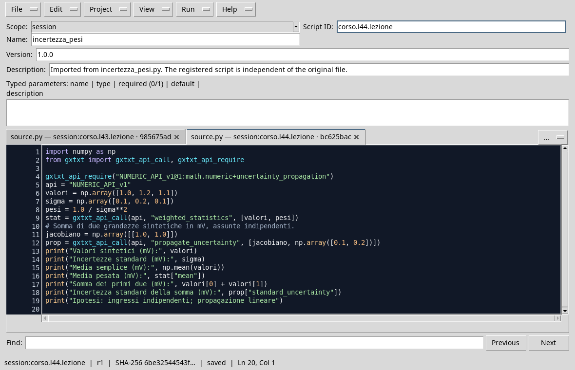
At the corso_python Session, import uncertainty_and_weights.py, save the script and run it in the Runner.
import numpy as np
from gxtxt import gxtxt_api_call, gxtxt_api_require

gxtxt_api_require("NUMERIC_API_v1@1:math.numeric+uncertainty_propagation")
api = "NUMERIC_API_v1"
values = np.array([1.0, 1.2, 1.1])
sigma = np.array([0.1, 0.2, 0.1])
weights = 1.0 / sigma**2
stat = gxtxt_api_call(api, "weighted_statistics", [values, weights])
# Sum of two synthetic sizes in mV, independent assumed.
jacobian = np.array([[1.0, 1.0]])
prop = gxtxt_api_call(api, "propagate_uncertainty", [jacobian, np.array([0.1, 0.2])])
print("Synthetic values (mV):", values)
print("Standard uncertainties (mV):", sigma)
print("Simple media (mV):", np.mean(values))
print("Average weighed (mV):", stat["mean"])
print("Sum of the first two (mV):", values[0] + values[1])
print("Standard uncertainty of the sum (mV):", prop["standard_uncertainty"])
print("Hypothesis: independent inputs; linear propagation")
weighted_statistics uses the values and weights provided. To propagate the uncertainty of the sum of the first two values, the Jacobian is [1, 1]: each partial derivative of the sum compared to an input is worth 1. Passing the two standard uncertainties, the calculation assumes a matrix of diagonal covariance, that is, covariance nothing between the two entrances in the example.
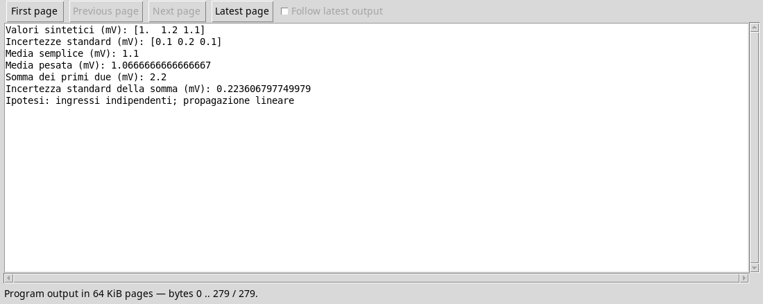
The simple average is 1,1 mV; the weighing average is about 1,067 mV. The sum is 2,2 mV and its standard uncertainty is \(\sqrt{0{.}1^2+0{.}2^2}\approx0{.}224\,\mathrm{mV}\). The unit of variance is mV2, while the standard uncertainty is in mV. The number of printed figures is used for numerical control: results and uncertainty are rounded in a relationship in a manner consistent with the stated accuracy.
Correction and limits
If the inputs are related, the term \(2\operatorname{cov}(x_1,x_2)\) appears for a sum. The API can receive a complete matrix of covariance with the appropriate option; it is necessary to provide consistent values and units. The propagation is of the first order: for strong nonlinear models or large uncertainties a different analysis may be necessary. A standard uncertainty is not automatically a range with a certain level of confidence.
Exercise
- What are the weights proportional to the three inverse variances?
- What is the sum of the first two values and its uncertainty in the hypothesis of independence?
- Why can’t we ignore a known covariance?
Worked solution
100,25,100in inverse units of variance; the ratio is4:1:4.2,2 mVwith standard uncertainty about0,224 mV.- It contributes to the variance of the result; ignoring it can substimate or overestimate uncertainty.
In the next lesson we will interpret tests and resamping without attributing to the p-value meanings that it does not have.