

Hypothesis Testing, Bootstrap and Inference Limits
Scientific Python in GX-TXT · Module 8 · Lesson 45
A statistical test assesses how much a result is compatible with a specified model and hypothesis. The bootstrap uses data resamping available to explore the variability of an estimate. Here we apply both to two small synthetic groups.
Objectives
- Define the difference between the means and state the null hypothesis.
- Run a bilateral Welch test in the numerical API.
- Generate a percentile bootstrap interval with explicit seed.
- Interpret the results without attributing to p-value improper meanings.
Two synthetic groups
The groups A and B contain five values each in mV, built for the exercise. We consider the difference mean_value(A) - mean_value(B) and the hypothesis nothing difference between averages equal to zero. The Welch test does not require the same variances between groups; however, it requires hypotheses on sampling and adequacy of the model. For the exercise we treat groups as independent.
Execution
At the corso_python Session, import bootstrap_test.py, save the script and run it in the Runner.
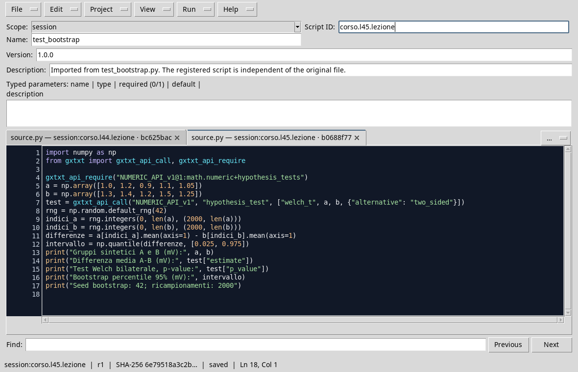
import numpy as np
from gxtxt import gxtxt_api_call, gxtxt_api_require

gxtxt_api_require("NUMERIC_API_v1@1:math.numeric+hypothesis_tests")
a = np.array([1.0, 1.2, 0.9, 1.1, 1.05])
b = np.array([1.3, 1.4, 1.2, 1.5, 1.25])
test = gxtxt_api_call("NUMERIC_API_v1", "hypothesis_test", ["welch_t", a, b, {"alternative": "two_sided"}])
rng = np.random.default_rng(42)
indices_a = rng.integers(0, len(a), (2000, len(a)))
indices_b = rng.integers(0, len(b), (2000, len(b)))
differences = a[indices_a].mean(axis=1) - b[indices_b].mean(axis=1)
interval = np.quantile(differences, [0.025, 0.975])
print("Synthetic groups A and B (mV):", a, b)
print("Average Difference A-B (mV):", test["estimate"])
print("Bilateral Welch Test, p-value:", test["p_value"])
print("Bootstrap percentile 95% (mV):", interval)
print("Seed bootstrap: 42; resamping: 2000")
The hypothesis_test API performs the welch_t bilateral test. The bootstrap is calculated locally with NumPy: for each of the 2000 foreign resampings with re-insertion indexes within each group, it calculates the two averages and saves the difference. The percentages 2.5% and 97.5% of the distribution thus obtained form the percentile range shown. The seed 42 makes this specific simulation repeatable in the same context.
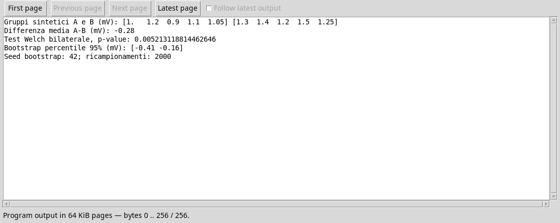
The difference observed A − B is -0,28 mV. The p-value of the test is about 0,0052; the bootstrap percentile interval shown is about [-0,41, -0,16] mV. These are different methods: the test and bootstrap interval are not the same procedure and are based on hypotheses. With so small samples the bootstrap can be unstable and does not automatically correct non-representative sampling or dependencies.
Correct interpretation
The p-value is the probability, under the hypothesis nothing and the other assumptions of the test, to obtain a statistics at least as extreme according to the rule of the test. It is not the probability that nothing is true, nor does it measure the practical importance of the difference alone. The interval should be interpreted in the context of the procedure and its hypotheses; it does not demonstrate a cause. In a real study it is necessary to consider drawing, independence, sample size, uncertainties and possible multiple comparisons.
Exercise
- What difference was calculated: A − B or B − A?
- What remains fixed in bootstrap resampings of this example?
- Is a p-value of 0.0052 the probability that nothing is true?
Worked solution
- A − B, equal to
-0,28 mVin the selected data. - The size of each group; the indices are extracted separately from the two groups.
- No: p-value is calculated by assuming the hypothesis nothing and the model of the test.
In the next lesson we will use the Curve Fitter on a published Dataset.