

Numerical APIs and Array Algebra
Scientific Python in GX-TXT · Module 5 · Lesson 25
In this lesson we compare two ways of calculating with the matrices: NumPy in the Python process and the GX-TXT numerical service, reached through the Bridge. We work with synthetic numbers and without physical units, chosen to make the result verifiable by hand.
What you’ll learn
- Recognize the shape and type of an array.
- Distinguish the product element by element from the matrical product.
- Request a function of the numerical API and read the result.
- Compare numerical results with tolerance.
Matrices and shapes
A matrix is a rectangular table. A (2, 2)-shaped array has two rows and two columns. The shape, o shape, is part of the contract of an operation: in the matrical product the number of columns of the first matrix must coincide with the number of rows of the second. The result has the rows of the first and the columns of the second.
In the example we use
A = [[1, 2],     B = [[2, 0],
     [3, 4]]          [1, 2]]
The top left element of A @ B is 1×2 + 2×1 = 4; the complete result is [[4, 4], [10, 8]]. In Python, A @ B indicates the NumPy matrix product. Instead, A * B multiplys the corresponding elements and A ** 2 elevates each element to the square. The three operations answer different questions.
An element-by-element operation can use NumPy broadcasting: for example A + 2 adds climbing to each element. NumPy can also combine more general compatible forms, but it is not necessary to assume that an external service adopts the same rules. For the array_binary operations of this API a scalar can expand on an array; two non-scale operators must have identical shape. Array operations described by the API accept real values with a maximum of two dimensions; invalid domains and unfinished values require attention. linear_matrix has a distinct contract and accepts non-black and finite real or complex matrices.
The full script
Open the corso_python Session, import array_algebra.py into the Python Script Workspace, assign him an ID and save him. Open Run → Open Script Runner and choose Run Job.
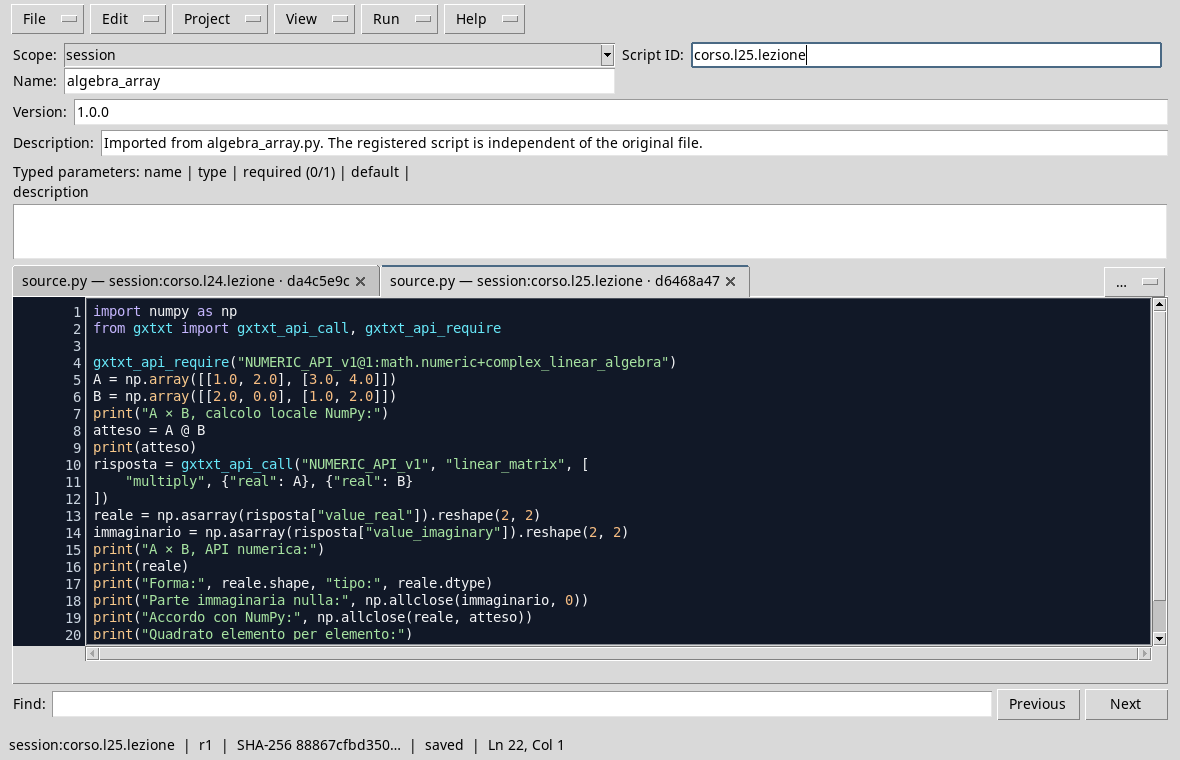
import numpy as np
from gxtxt import gxtxt_api_call, gxtxt_api_require

gxtxt_api_require("NUMERIC_API_v1@1:math.numeric+complex_linear_algebra")
A = np.array([[1.0, 2.0], [3.0, 4.0]])
B = np.array([[2.0, 0.0], [1.0, 2.0]])
print("A × B, local calculation NumPy:")
expected = A @ B
print(expected)
response = gxtxt_api_call("NUMERIC_API_v1", "linear_matrix", [
    "multiply", {"real": A}, {"real": B}
])
real_part = np.asarray(response["value_real"]).reshape(2, 2)
imaginary = np.asarray(response["value_imaginary"]).reshape(2, 2)
print("A × B, Number API:")
print(real_part)
print("Forma:", real_part.shape, "tipo:", real_part.dtype)
print("No imaginary part:", np.allclose(imaginary, 0))
print("Agreement with NumPy:", np.allclose(real_part, expected))
print("Element square by element:")
print(A ** 2)
gxtxt_api_require checks that the requested provider has a complex linear algebra capacity. It is a preventive verification: it does not calculate the product. gxtxt_api_call instead sends the request to the NUMERIC_API_v1 service, specifying the linear_matrix operation, the multiply action and the two operators. The {"real": A} and {"real": B} dictionaries represent real matrices; the contract can also represent the imaginary part.
The answer separates value_real and value_imaginary. Here we reassemble each part in the (2, 2) waiting form, specific of this example. In a general program the form must be obtained and verified according to the contract and the size of the inputs, without always fixing 2×2. We also print the dtype, i.e. the numerical type of the elements: in the performance shown is float64.
Read and check the result
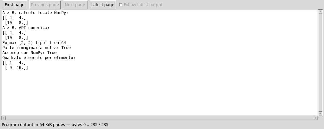
The Job prints [[4, 4], [10, 8]] for both calculations. The imaginary part is nothing and np.allclose returns True. This comparison uses tolerances, appropriate because two implementations in mobile comma can differ from a small amount. For a real application, choose rtol and atol based on the accuracy and scale of data; approximate equality does not replace unit control.
The NumPy calculation takes place in the Python script; the request to the Bridge uses the GX-TXT numerical provider. Even when results coincide, entrance contracts, context and costs can be different. The matrical call treats numbers as mathematical values: if they represent physical quantities, it is up to those who write the program to check that the units are compatible and attribute the correct ones to the result.
Try it.
- Before performing, calculate by hand
A ** 2andA @ B. Why are they different? - Replace
Bwith the[[1.0, 0.0], [0.0, 1.0]]identity matrix and verify that the product returnsA. - Imagine a
Cmatrix with(3, 2)shape: can you calculateA @ C? What aboutC @ A? Indicates the form of the admitted result.
Worked solution
A ** 2produces[[1, 4], [9, 16]]: each element is elevated to the square.A @ Binstead combines rows and columns and produces[[4, 4], [10, 8]].- The identity matrix leaves the product unchanged: with
np.allclose(real_part, A)you getTrue, within the tolerance used. A @ Cis not defined because the two internal dimensions are 2 and 3.C @ Ais defined: the internal dimensions are both 2 and the result is(3, 2)shape.
In the next lesson we will use a grid to estimate intermediate values of a curve, distinguishing estimates from the observed data.