

The First 2D Curve in the GX-TXT Viewer
Scientific Python in GX-TXT · Module 6 · Lesson 32
We create a persistent chart from a Canon Dataset of the Session. We will use the PlotSpec prepared in the previous lesson and we will ask GX-TXT to render the synthetic series of the course.
Objectives
- Associate an ascissa and an order to a series.
- Validate the spec, create a variant and request rendering.
- Open the result in the GX-TXT graphics window and read the axes.
- Distinguish the graphic object from the source data and the image displayed.
Data and choice of axes
The corso_python_serie_sintetica series contains four synthetic pairs: 0 time, 0,5, 1, 1,5 s and 1,2 signal, 1,5, 1,3, 1,6 mV. In this example the time is the horizontal coordinate, while the signal is the vertical coordinate. line_marker shows the points and connects them with segments: the link helps reading, but does not transform intermediate values into measures.
Create chart
In the corso_python Session, import first_curve.py, save the script in the Python Script Workspace and start it with Run → Open Script Runner → Run Job.
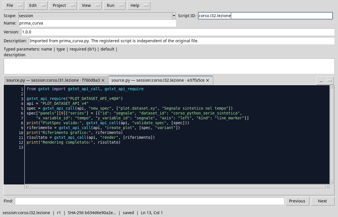
from gxtxt import gxtxt_api_call, gxtxt_api_require

gxtxt_api_require("PLOT_DATASET_API_v4@4")
api = "PLOT_DATASET_API_v4"
spec = gxtxt_api_call(api, "new_spec", ["plot.dataset.xy", "Synthetic signal in time"])
spec["panels"][0]["series"] = [{"id": "segnale", "dataset_id": "corso_python_serie_sintetica",
    "x_variable_id": "tempo", "y_variable_id": "segnale", "axis": "left", "kind": "line_marker"}]
print("PlotSpec valid:", gxtxt_api_call(api, "validate_spec", [spec]))
reference = gxtxt_api_call(api, "create_plot", [spec, "variant"])
print("Graphic reference:", reference)
result = gxtxt_api_call(api, "render", [reference])
print("Complete Rendering:", result)
Validation controls the specification. create_plot creates a variant and returns a reference; render uses that reference to generate representation. Keep the identity returned if you need to reopen or change the same chart. Every new creation of a variant can produce a different identity.
In the GX-TXT Plots tab, select the variant created. The graph appears in the preview; by double-clicking the image you can open it in the graphics window and use the adjustment and zoom commands.
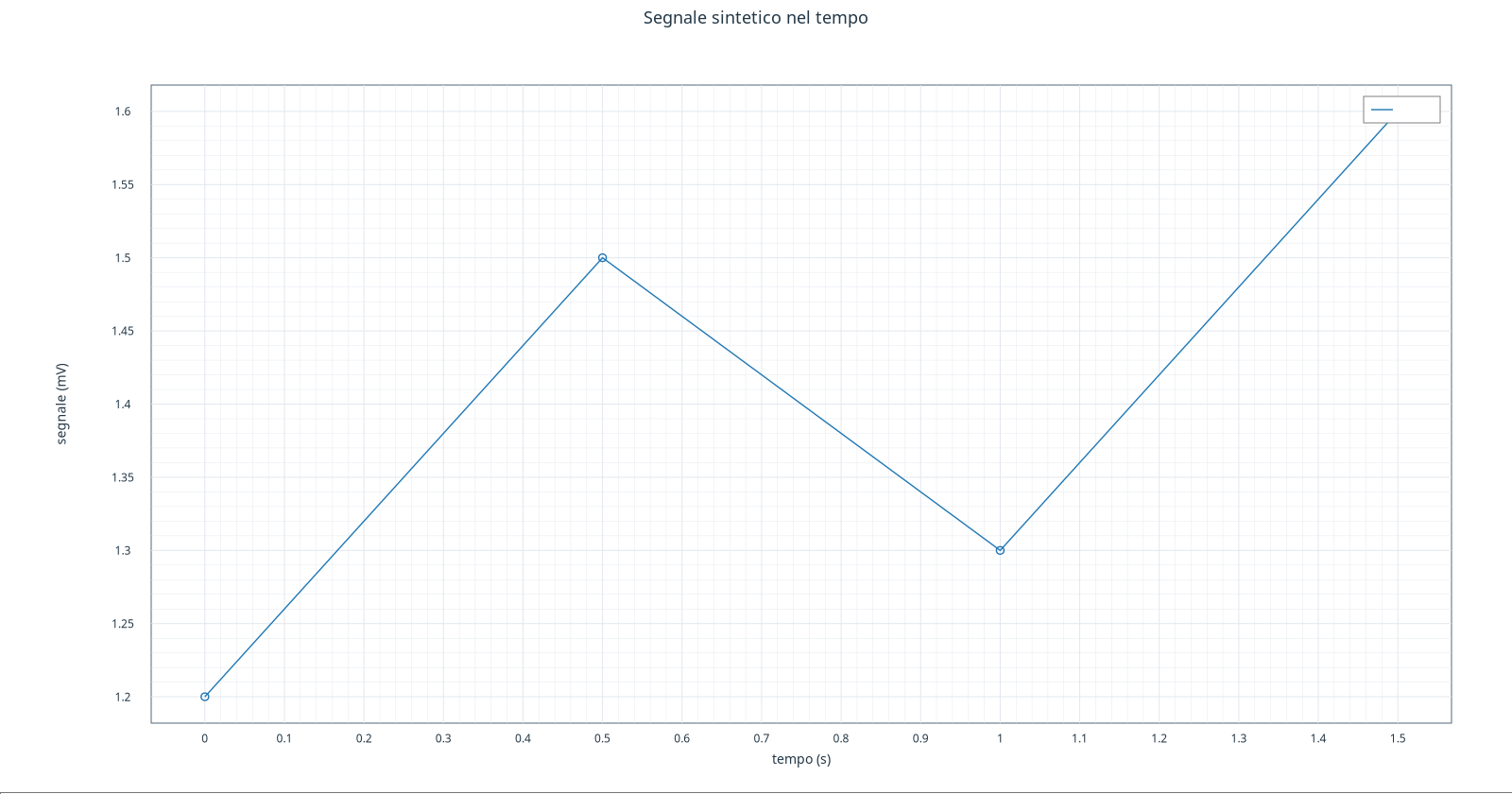
Note on the version. The guide was made with GX-TXT dev112-P011-bis. In this version, the option to hide the legend in the
native_presentationcan prevent the creation of the graph even when the specification is valid. This is why a screenshot of the curve with the hidden legend is not available: the figure above shows the actual rendering with the default configuration, in which the legend covers the last point. The expected behavior is to show the complete curve without legend when choosingplacement: none. According to the indication given for the course, the problem is corrected in dev112-P012 and in subsequent versions; the correction was not verified on this installation P011-bis.
The title indicates that it is synthetic data. Axle labels report variable units. The image is a representation of the Dataset: it does not replace the data, IDs or choices of the spec. If the labels or the layout are not readable, in the next lesson we will see how to intervene on the options of the chart.
Check reading
At 0,5 s the series reaches 1,5 mV; at 1 s it descends to 1,3 mV. The vertical scale shown is adapted to the data, so it does not necessarily start from scratch: when different graphic comparisons controls the limits of the axes, in addition to the shape of the line.
Exercise
- Which fields of the series choose X and Y?
- What is the synthetic value at
1 s? - Does the segment between two points prove that all intermediate values have been measured?
Worked solution
x_variable_idandy_variable_id,time_valuesandsignalrespectively.1,3 mV.- No. The segment is a graphic choice that connects available points; intermediate values do not become new measures.
In the next lesson, we’ll have titles, units and scales.