

Curve Fitter Models and Results
Scientific Python in GX-TXT · Module 8 · Lesson 46
The Curve Fitter allows you to adapt a model to a curve of a Dataset and to examine parameters and residuals. In this lesson we use an exact linear synthetic series, so as to compare the result with the known parameters.
Objectives
- Load a curve from a Dataset and choose a model.
- Distinguish preview and fit accepted.
- Read parameters, units, residues and method status.
- Consult the catalogue of available models from Python.
Load the curve
Open the corso_python Session, select Viewers → Curve Fitter, choose the Dataset corso_python_seconda_serie, X time_values (s) and Y signal (mV), then Add Dataset curves. This Dataset was created in lesson 34 and contains four synthetic points on the \(y=1+0{.}2t\), with y in mV and t in s.
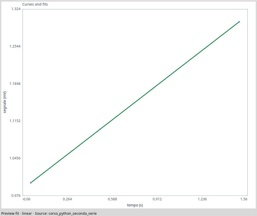
Select the curve in the source list and choose Fit → Preview fit. The linear model of this example produces the following preview. To store the fit use Fit → Accept fit, assign a name and save the Workspace.
Parameters and residues
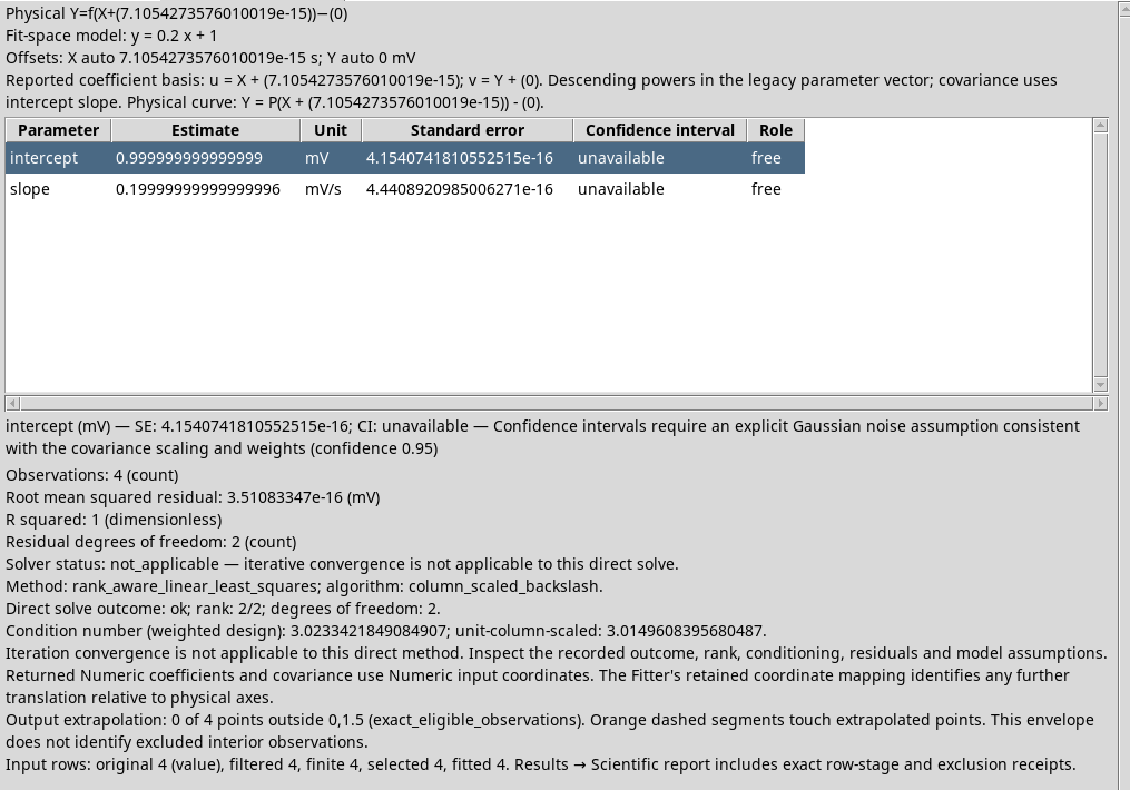
Open Parameters & Statistics. The intercept is about 1 mV and the gradient about 0,2 mV/s, as provided by the formula that generated the data. The method indicated is a direct linear solution: the status of iterative convergence is indicated as non-applicable. It should not be described as a convergent iterative solver.
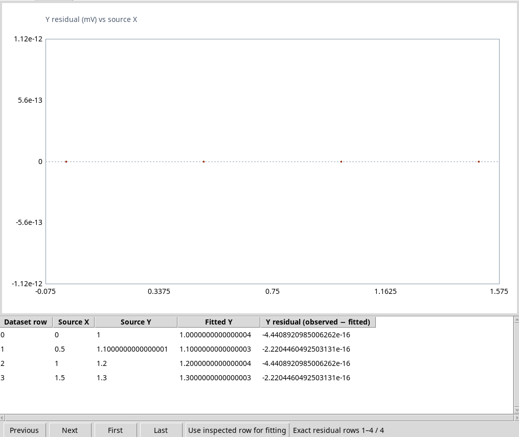
In the Residuals tab, the residue is given by less predicted observed. In this ideal example the residues are close to zero to numerical accuracy: the data were built exactly on the same straight. This situation does not show that a linear model is always appropriate for experimental data.
Catalogue of Python models
The following Download the Module 8 scripts (ZIP) questions model tabs and the Session Workspace list. Import it into the Python Script Workspace and start it in the Runner.
from gxtxt import gxtxt_api_call, gxtxt_api_require

gxtxt_api_require("DATASET_CURVE_FIT_API_v1@1")
gxtxt_api_require("SESSION_WORKSPACE_API_v1@1")
models = gxtxt_api_call("DATASET_CURVE_FIT_API_v1", "model_cards", [])
workspace_list = gxtxt_api_call("SESSION_WORKSPACE_API_v1", "list", [])
print("Available templates:", len(models))
print("Session Workspace:", len(workspace_list))
for workspace in workspace_list:
    print("Workspace:", workspace.get("id"), workspace.get("name"), workspace.get("provider_id"))
In the performance shown, the API returns 22 tabs and a Workspace by Curve Fitter. A public recipe captured by an accepted fit allows you to describe and repeat an analysis explicitly; you need to use the identity of the result and verify the source and version before the reuse.
Note on the version. In the dev112-P011-bis copy used for driving, the generic reading of Curve Fitter’s Workspace through
SESSION_WORKSPACE_API_v1/getreturned a transport error (unsupported provider result type Tcl_Obj). This is why we do not show a screenshot of the recipe acquisition through that reading. The expected behavior is to return the Workspace with transferable data to the client, so that it can continue with public operations on the results. The correction has not been verified in this installation; the version in which it will be available must be confirmed on the actual release.
Exercise
- What units have intercepted and sloped?
- Why are the residues almost null in the example?
- Why doesn’t the status ‘non-applicable fisheries convergence’ automatically mean that the fit has failed?
Worked solution
- The intercept is in mV; the slope in mV/s.
- The four synthetic points were built on a straight; small numerical gaps remain.
- The method shown is a direct solution, not an iterative algorithm: the outcome of the solution must be read together with the parameters and the residues.
In the next lesson we will compare different models on the same data.