

Comparing Models and Residuals
Scientific Python in GX-TXT · Module 8 · Lesson 47
A more complex model is not automatically better. We face a first-degree polynomial and a second-degree polynomial on the same four synthetic points, observing residues and degrees of freedom.
Objectives
- Adapt two nested models to the same data.
- Read coefficients, residues and sum of squares.
- Consider the number of parameters and degrees of freedom.
- Distinguish numerical adaptation and physical plausibility.
Execution
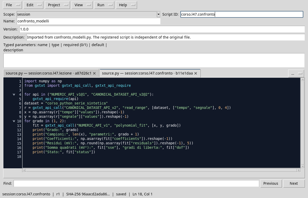
The Dataset corso_python_serie_sintetica contains four didactic values, not measures. At the corso_python Session, import model_comparison.py, save the script and run it in the Runner.
import numpy as np
from gxtxt import gxtxt_api_call, gxtxt_api_require

for api in ("NUMERIC_API_v1@1", "CANONICAL_DATASET_API_v2@2"):
    gxtxt_api_require(api)
dataset = "corso_python_serie_sintetica"
r = gxtxt_api_call("CANONICAL_DATASET_API_v2", "read_range", [dataset, ["tempo", "segnale"], 0, 4])
x = np.asarray(r["tempo"]["values"]).reshape(-1)
y = np.asarray(r["segnale"]["values"]).reshape(-1)
for degree in (1, 2):
    fit = gxtxt_api_call("NUMERIC_API_v1", "polynomial_fit", [x, y, degree])
    print("Grado:", degree)
    print("Samples:", len(x), "parametri:", degree + 1)
    print("Coefficienti:", np.asarray(fit["coefficients"]).reshape(-1))
    print("Residui (mV):", np.round(np.asarray(fit["residuals"]).reshape(-1), 5))
    print("Square sum (mV2):", fit["sse"], "degrees of freedom:", fit["dof"])
    print("Stato:", fit["status"])
The for cycle requires the polynomial_fit API 1 and 2 degrees on the same X and Y values. The first model has two coefficients, the second three. The second contains the first as a special case when the square coefficient is zero: they are nested models. The API returns coefficients in descending order of powers, residues, sum of squares and information on the solution.
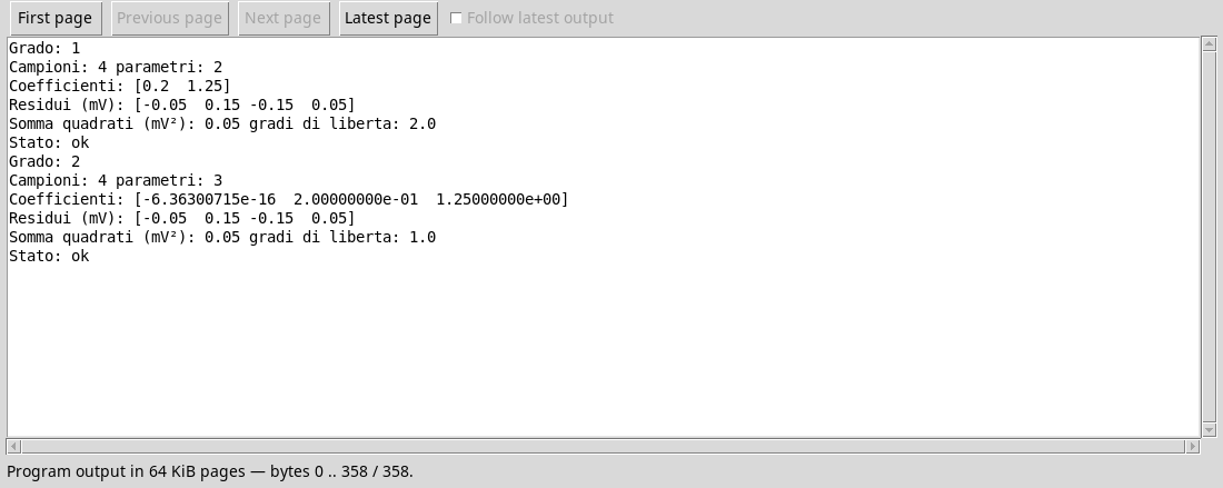
In this execution both have sum of the residual squares of approximately \(0{.}05\,\mathrm{mV}^2\). The square coefficient is practically zero to numerical accuracy, so the expected values coincide with those of the straight. Grade 1 model has two degrees of residual freedom; grade 2 has one. Adding a parameter did not improve the adaptation on this data.
Interpreting comparison
The sum of the squares is a measure of disagreement on the data used for the fit, but it does not tell everything. More parameters can also adapt to noise: it is the risk of overfitting. For a serious comparison use the same data and weights, check residues, conditioning and hypotheses, and choose criteria suitable for sample size. With four points there is no need to generalize strong conclusions. A better numerical metric does not show that a model correctly describes the physical phenomenon.
Exercise
- How many parameters does each polynomial have?
- What does the near-zero square coefficient suggest in this example?
- Why do we compare the two models on the same observations?
Worked solution
- Two for grade 1 and three for grade 2, including intercept.
- That the second degree term does not add an appreciable curvature in the shown fit.
- In order to compare residues and metrics: changing data or weights would also change the problem.
In the next lesson we will build a relationship that distinguishes estimates, uncertainties and conclusions.