

Plots, Session and integrated report
Scientific Python in GX-TXT · Module 10 · Lesson 59
We visualize together synthetic data and curves obtained from fits. The figure compares the two conditions; the numerical report from the previous lesson remains necessary to read convergence and residuals.
Objectives
- Compose a spec with four series from separate Dataset.
- Distinguish synthetic points and fit curves in the legend.
- Read axes and units without confusing data and pattern.
- Read the plot alongside the numerical diagnostics.
Execution
After Lessons 56 and 58, import final_plot.py, save it and start it at the corso_python Session.
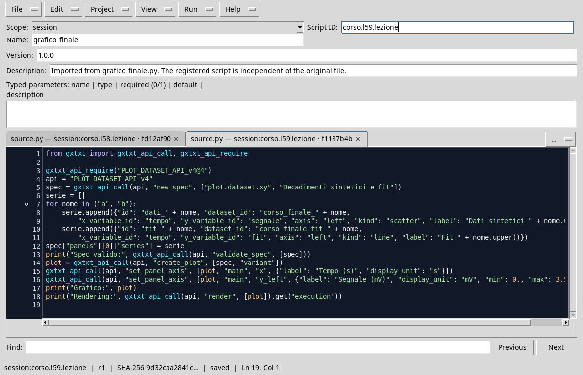
from gxtxt import gxtxt_api_call, gxtxt_api_require

gxtxt_api_require("PLOT_DATASET_API_v4@4")
api = "PLOT_DATASET_API_v4"
spec = gxtxt_api_call(api, "new_spec", ["plot.dataset.xy", "Synthetic decay and fit"])
series = []
for display_name in ("a", "b"):
    series.append({"id": "dati_" + display_name, "dataset_id": "corso_finale_" + display_name,
        "x_variable_id": "tempo", "y_variable_id": "segnale", "axis": "left", "kind": "scatter", "label": "Synthetic " + display_name.upper()})
    series.append({"id": "fit_" + display_name, "dataset_id": "corso_finale_fit_" + display_name,
        "x_variable_id": "tempo", "y_variable_id": "fit", "axis": "left", "kind": "line", "label": "Fit " + display_name.upper()})
spec["panels"][0]["series"] = series
print("Expenditure valid:", gxtxt_api_call(api, "validate_spec", [spec]))
plot = gxtxt_api_call(api, "create_plot", [spec, "variant"])
gxtxt_api_call(api, "set_panel_axis", [plot, "main", "x", {"label": "Tempo (s)", "display_unit": "s"}])
gxtxt_api_call(api, "set_panel_axis", [plot, "main", "y_left", {"label": "Segnale (mV)", "display_unit": "mV", "min": 0., "max": 3.5}])
print("Graph:", plot)
print("Rendering:", gxtxt_api_call(api, "render", [plot]).get("execution"))
The loop builds for each condition a series of points from the Synthetic Dataset and a line from the Dataset of the fit. The series list contains four dictionaries. The labels identify data and model; the axes show time in seconds and signal in millivolts.
In the Plots tab, select the created variant and open the figure. The following capture comes from the GX-TXT graphic window, adapted to the window and cut out to remove the external contour.
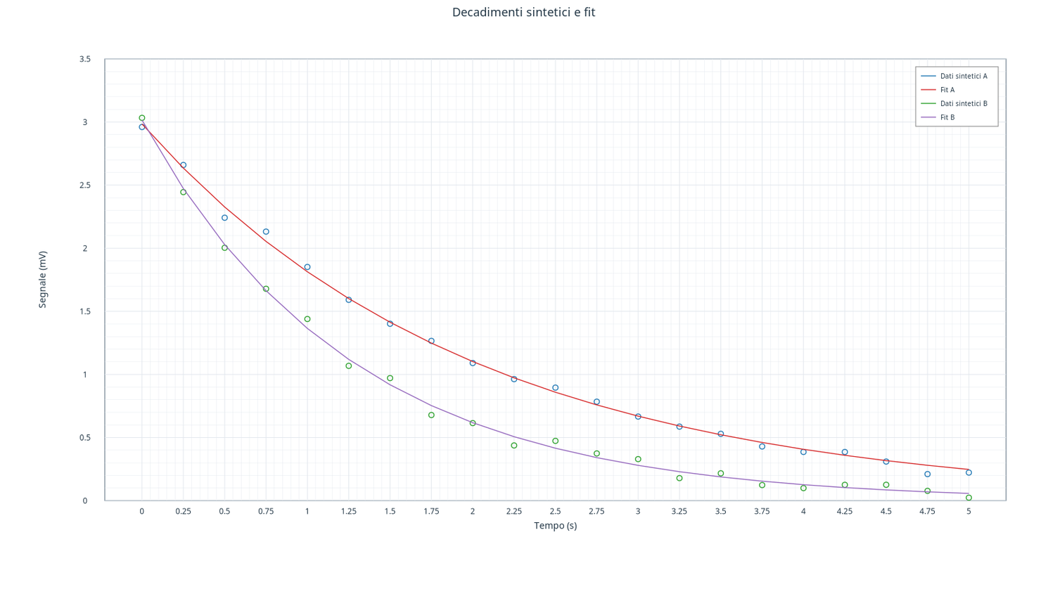
The two sets of points are synthetic: they do not represent measurements. The lines are model predictions on the published times. The B condition decays more quickly, as provided by the generation parameters; the deviations of the points from the curves reflect the synthetic noise.
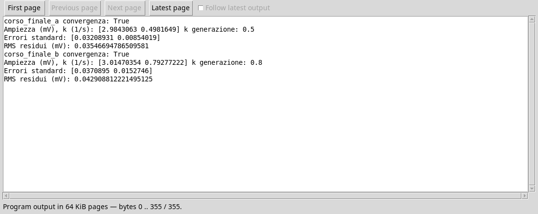
The figure does not replace the verification of the solver and the residuals. In the associated relationship states Dataset, seed, model, parameters, units, uncertainties and limits. The notes of the original Dataset retain the synthetic protocol; the fit curves are published as separate Dataset derivatives.
Exercise
- How many series make up the chart and which ones are predictions?
- What condition decays faster?
- Why is visual agreement alone not enough to certify a fit?
Worked solution
- Four: two sets of synthetic data and two fitted curves.
- B, which has the larger decay constant.
- Convergence, residues, hypotheses and uncertainties must be checked in addition to the figure.