

Mediterranean and Climate · Data and Methods
Series to download
- Temperature and anomaly 1926–2025 · Recent window · Cells and weights.
- Sea–air comparison · Pairs for the fit · Year-on-year differences.
- Temperatures at five depths, XYZ + temperature · Three vertical profiles.
- Bathymetry, thinned XYZ grid · Original NetCDF subset from the NOAA server (NetCDF .nc file in a ZIP archive).
Repeating the plots and the regressions
Import the CSV files with Generic CSV dataset import. For the century plot in Curve Viewer bind anno and anomalia_c. For the comparison use anno and two sources with mare_c and aria_media_tre_c. In Curve Fitter choose the linear, all points and Preview fit. Repeat for each time window. For the sea–air relationship bind the anomaly columns to each other, then the year-on-year difference columns. If other curves are present in the window, select the intended source before running the Preview. For the slopes use Parameters & Statistics. Converting to degrees per decade multiplies the annual slope by ten.
Creating the two 3D views
- In Curve Viewer choose New 3D → Add source…. Bind X to
longitudine, Y tolatitudine, Z toquota_m. For the bathymetry, select both elevation bindings, Z and Independent scalar C Variable. For temperature choosetemperatura_c. - In the Plot tab use
scatter3. Press Apply and wait for Native3D draft ready. Use Fit, then drag the plot to change the viewpoint. - For the plan view in the figure, select the 3D root and open Native camera… in the Inspector. Set projection to
orthographic, camera position to0;0;2.85, camera target to0;0;0, camera up to0;1;0, near clip to0.4and far clip to8. The coordinates of the camera module are normalized in the viewer scene.
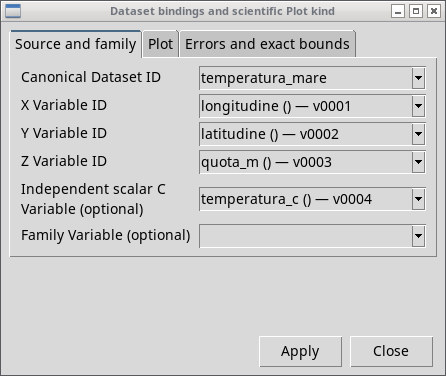
The identifiers after the dash in the lists can take values such as v0001. Identify the column by the name in the CSV. In 3D the visual scaling makes quantities with different units readable. Measuring a physical length or slope requires an appropriate projection and scale.
Sources, preparation and reuse
- Surface. NOAA PSL, ERSST v5. NCSS subset with
sst, geographic bounds 7°W…38°E and 29°…47°N, months from January 1926 to December 2025. To build the 58 cells, the Natural Earth mask was applied to the centers with complete monthly coverage. The script was needed to read the time and grid of the NetCDF together, apply the geometries, weight cells and months, and prepare a CSV for the viewer. NOAA catalog and download · Natural Earth reuse. - Depth. NOAA World Ocean Atlas 2023, Volume 1, field
t_an, annualt00, 1°, 1991–2020 normaldecav91C0. The script selects the values available in the marine cells, the required levels and the three profiles from the NetCDF 4 array. The reduced CSV is attached; the global original can be downloaded from the catalog. NOAA distribution · Original file and access options. - Bathymetry. EMODnet Bathymetry Consortium, DTM 2024,
elevationrelative to Lowest Astronomical Tide. Polygon filtering, thinning from 0.25° to 0.5° and conversion to XYZ rows were done before using Curve Viewer. The dataset metadata allow redistribution of the data. Original ERDDAP query · License and attribution. - Air. Data obtained from the NASA POWER project funded by the NASA Earth Science Applied Sciences program. Extraction
T2M,AG, annual series 1981–2025 at the points Valencia (−0.53°, 39.53°), Rome (12.48°, 41.89°), Athens (23.735°, 37.98°). The script aligns years and units, computes the anomalies and prepares the paired inputs for Curve Fitter. API and definitions · NASA POWER attribution.