

Cells, sheets, and formatting
Edit and copy cells, fill ranges, and manage formats, sizes and merged cells with the manual’s examples.
Select and move around the grid
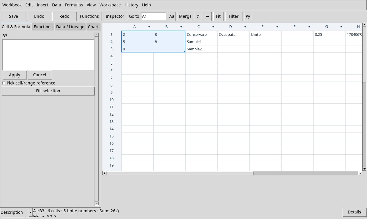
Start with a test Workbook and click A1. Paste the TSV exercise block (unzip the archive first) from the clipboard. The highlighted border marks the current target. Cell & Formula shows the address you are editing. The status bar shows the rectangle, the number of cells and, for compatible selections of up to 5,000 cells, a summary of the finite numbers.
- Click, drag and Shift+click
- A click replaces the selection with a single cell. Press in the body of A1, drag to B3 and release to get A1:B3. With Shift+click on D2 the rectangle starts from the anchor A1. Ctrl+click on C3 selects only C3. The grid works with a single contiguous rectangle. If Shift+Up arrow creates a range with inverted ends, start again from the upper cell and drag downwards.
- Row and column headers
- Press on the row number or column letter, away from the divider and the filter symbol. In the verified patch, the whole row or column is selected while you press. On release, the selection shrinks to the first relevant visible cell. To act on a precise stretch, select the cells in the body. To resize the whole row or column, one cell in the desired position is enough. The icon in the header opens the quick filter.
- Arrows, Shift and Ctrl+A
- The arrow keys move the active cell. Shift+arrow extends the rectangle from the anchor. Ctrl+A selects the envelope of the populated cells, A1:I3 in the initial exercise. Always check both corners before a destructive command.
- Tab, Shift+Tab, Enter
- Start with the grid active. Tab moves to the right and Shift+Tab back to the left. Enter moves down one row. In the D5 → D4 test, Shift+Enter instead left D5:D4 with a summary error. Use Up arrow to move up one row with a single selection.
- Home, End, Ctrl+arrows, Ctrl+Home, Ctrl+End
- Home and End go to the first and last available address in the row. Ctrl+arrow jumps to the current edge in the direction pressed. Ctrl+Home returns to A1 and Ctrl+End goes to the bottom-right corner of the available extent. The extent grows as you navigate and can include empty cells.
- Page Up, Page Down, scrolling, Go to
- Page Up and Page Down move the selection by the height of the pane. Use the mouse wheel to scroll vertically, Shift+wheel to scroll horizontally, or the scroll bars in both directions. The command target remains the selected one. To go directly to a cell, type
B2in Go to and press Enter.
Type, correct and recalculate
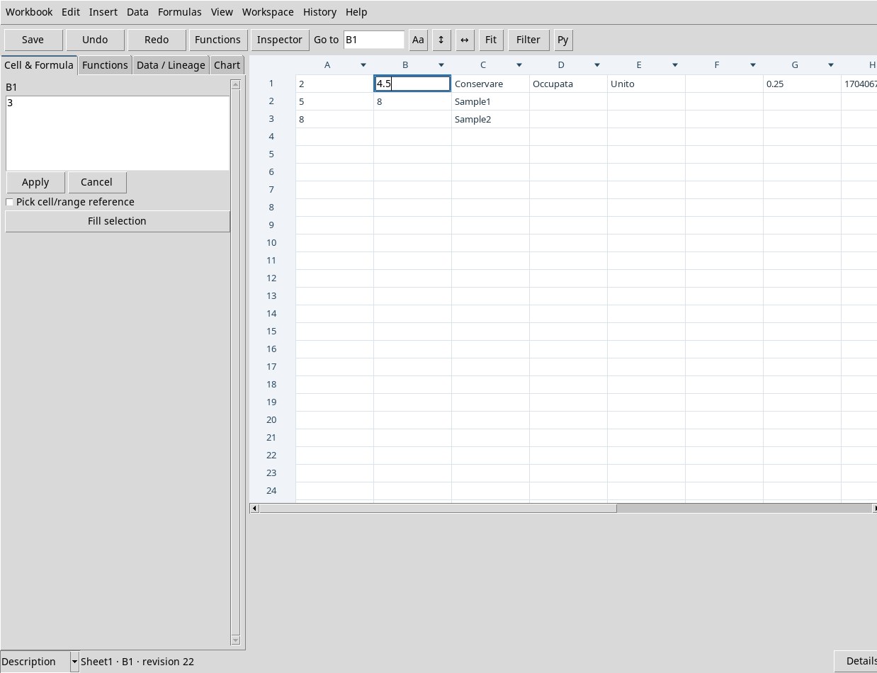
- Select B1. Type to replace the content. Double-click or press F2 to open the current source in the grid editor. With Esc to close the editor and discard the change.
- Type
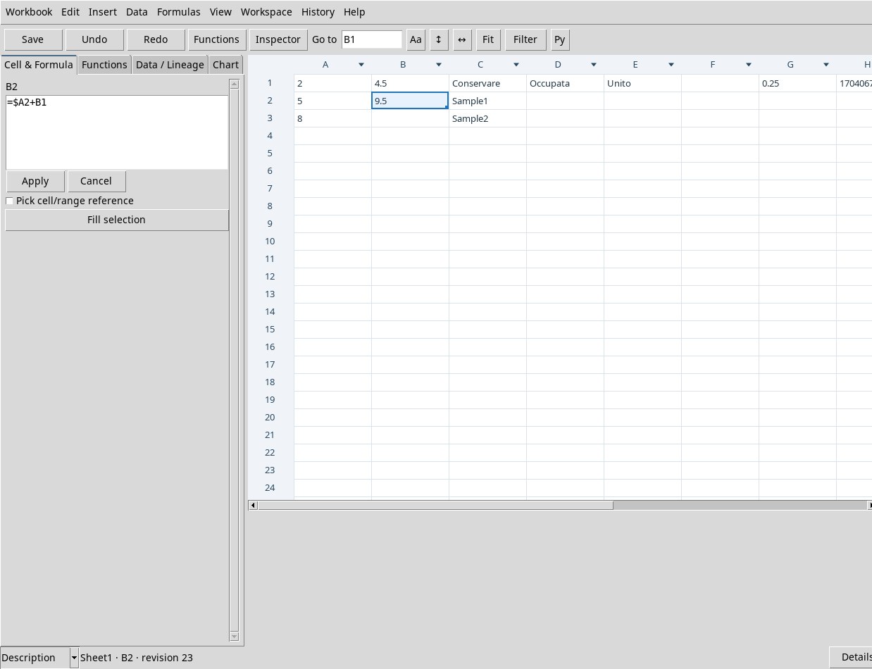
4.5and press Enter. The change is confirmed and the selection moves on. Tab and Shift+Tab confirm and move right and left respectively. B2 contains=$A2+B1and updates to 9.5 with automatic calculation. - For a long formula, a reference or multi-line text, open Cell & Formula. Check the address above the text area. Apply or Ctrl+Enter confirms. Cancel discards the edited text. Pick cell/range reference and Ctrl+Space help you insert references and functions.
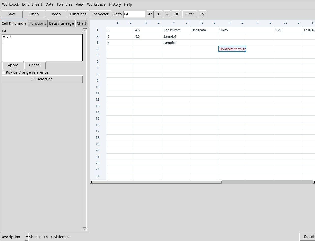
- Compare a formula shown in the editor with the value or message in the grid.
=1/0produces an error that you can inspect in the cell. Another formula can depend on the numerical result of B2.
The right mouse button opens the cell context menu. From here you can copy, paste, clear, fill, format, merge or split, adjust sizes and open Filters or Scripts. Check the target and the enabled items. Edit → Clear, Delete and the context menu clear the selected cells. References to a cleared value may become errors. Undo restores the value and the calculation, Redo repeats the action. When you make a change from an earlier History step, the dialog asks whether to discard the later local steps. Read the confirmation before choosing OK. See the History steps.
Copy, cut and paste
- Typed copy and paste
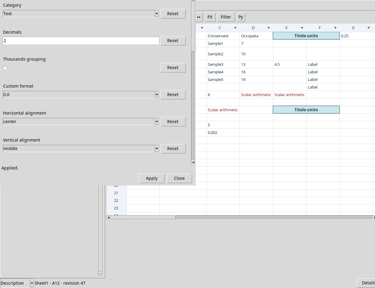
- Select the source and use Edit → Copy or Ctrl+C. Choose the top left cell of the destination and use Paste or Ctrl+V. The Worksheet clipboard keeps the formula source and shifts relative references. From A10 to B10
=A1+$B$1becomes=B1+$B$1. A cell already present at the destination can be overwritten. The typed format also transfers the style, as verified by copying to G2 the 0.25 formatted as a percentage in G1. Check units and formats when the target has already been prepared. - Cut and paste
- Cut or Ctrl+X places the block on the clipboard and immediately clears the source. Paste from B10 into C10 to get
=C1+$B$1, with the absolute reference preserved. Cut and paste generate two steps: the first Undo removes the paste and the second restores the source. - Text from another program
- Each tab outside quotes starts a new column, and each line break outside quotes starts a new row. With a quoted TSV, enclose the field in
"to include a tab or a line break, and double any quote inside it. A source that starts with=is evaluated at the coordinates where you paste it. In the test,01and2e-3are both scalars and keep their source text in the editor. A quoted field containing an internal line break remains a single cell. The exchange limit is 2 MiB.
Drag, fill and transfer ranges
To select, drag starting from the body of the cell. Even with Ctrl held down, the A1:D4 test produced a rectangle without transferring values. To move and copy a block, use the clipboard commands. To change widths and heights, start from the header divider.
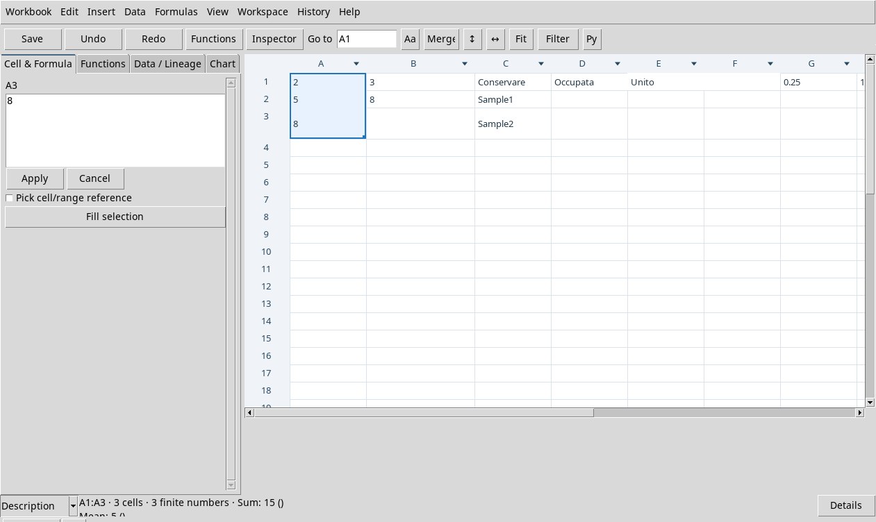
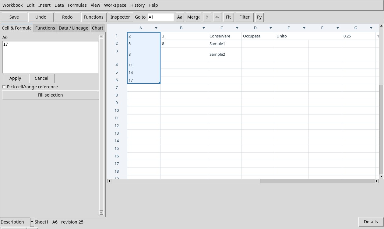
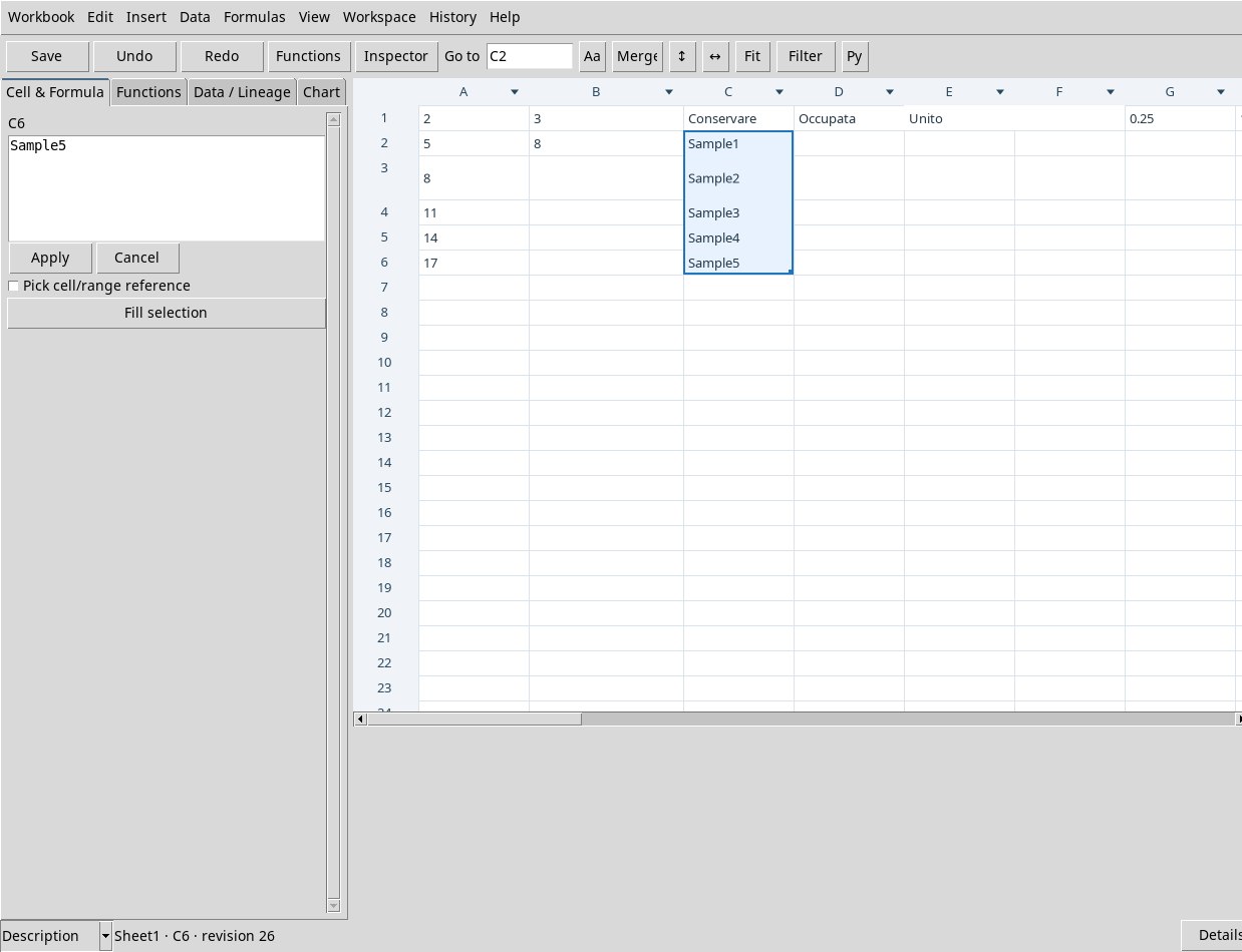
- Select A1:A3, which contains 2, 5, 8. Point to the small square at the bottom right of the selection. Drag the handle to A6 and release. A4:A6 receives 11, 14, 17 and the selection extends. Repeat from C2:C3 to C6 to get Sample3, Sample4, Sample5.
- Try a formula by writing
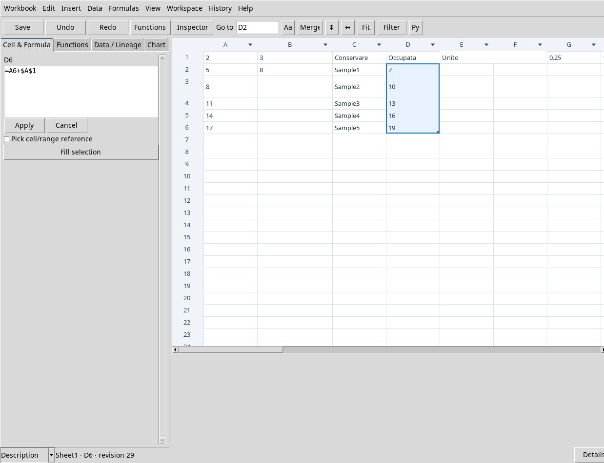
=A2+$A$1in D2 and a text in D3. Drag the D2 handle to D6. The text in D3 is replaced by=A3+$A$1. D6 receives=A6+$A$1and equals 19. The source cells remain part of the selection. - Edit → Fill down and Fill selection in Cell & Formula propagate from the first selected row. Fill right starts from the first column. For example, select B8:E8 with
=A1+$B$1in B8. The first copy uses B1. Later positions that refer to text produce an arithmetic error. Use a single column for Fill down or a single row for Fill right. In the patch, on A1:C3 both commands propagate A1 to all selected cells. To keep one source per column or per row, apply the command separately to each strip.
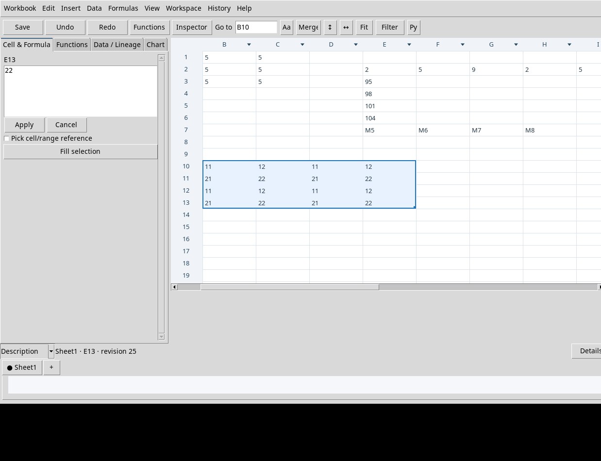
To stop the extension, bring the handle back to the starting edge before releasing. A7 stayed empty in the test. For a sequence with irregular increments, the handle repeats the block, as in 2, 5, 9, 2, 5, 9. Dragging upwards from 101, 104 gives 95 and 98 in the two cells above. Dragging to the left from M7, M8 gives M5 and M6. A rectangular source repeats as a two-dimensional block. If the drag enters a merged region, the Viewer may ask you to split the region before changing the cells beneath it. Check the status and the source data before trying again.
Insert rows, columns and sheets
With a cell active, open Insert. Insert row and Insert column insert at the active position and shift the following data. Delete row and Delete column remove the active position and close the gap. Check the affected formulas and ranges after a structural change. Use Undo to make a reversible test.
- New sheet… or +
- Opens Sheet name. Type a name and press Apply. Click a tab at the bottom to switch between sheets.
- Rename sheet…
- Renames the active sheet. Use unique names and check any references that name it.
- Duplicate sheet…
- Creates a worksheet with the contents of the active sheet. Give it a new name to keep a parallel experiment.
- Delete sheet
- Check that the dot is on the right sheet and read the confirmation. OK deletes the sheet. Cancel keeps it. A source Dataset remains a resource of the Session.
Format the appearance of cells
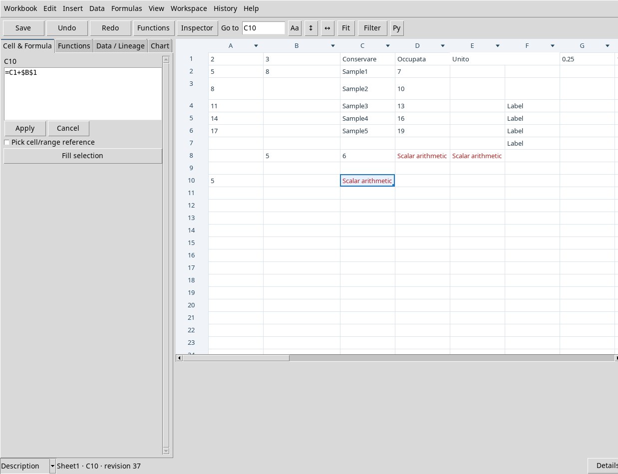
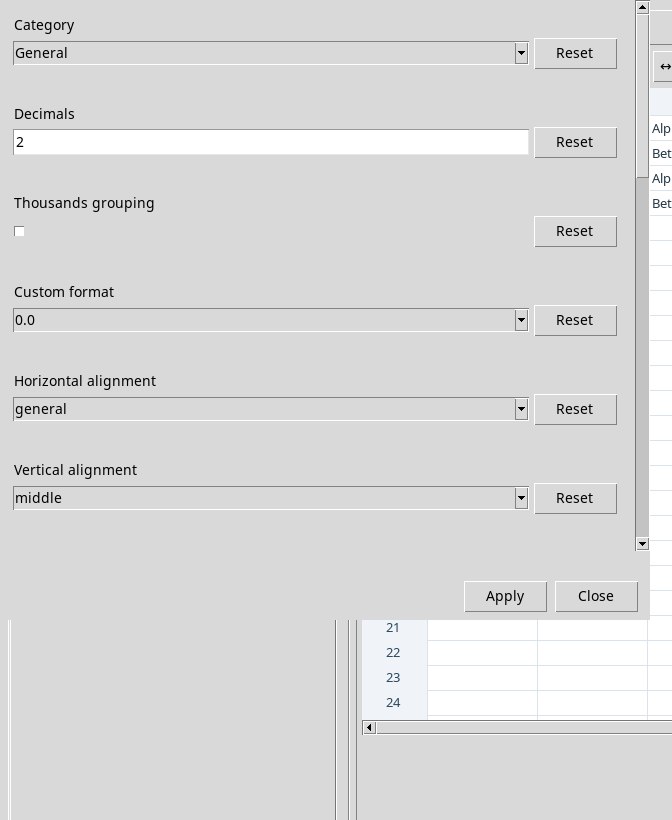
Select the rectangle, then open Edit → Format Cells, the Aa button, or the item of the same name in the context menu. The dialog starts from the style of the first cell. Change the fields and press Apply. Reset next to a field restores its default value in the draft. The test reset Category to General, Decimals to 2 and Wrap text to off. Close closes the dialog. An out-of-range value, for example 18 in Decimals, shows the limit next to the field. Formatting affects the displayed text, while the scientific values and units are kept.
- Category
Generaluses the ordinary display.Numberuses fixed decimals,Scientificshows the exponent,Engineeringuses exponents that are multiples of three, andPercentageshows the value scaled as a percentage.DateandTimedisplay Unix seconds as a date and a time. 1704067200 gives 2024-01-01 and 00:00:00.Textkeeps a text appearance.Customuses the chosen pattern.- Decimals, Thousands grouping, Custom format
- Decimals range from 0 to 17, initially 2. Grouping separates thousands in compatible formats. In Custom choose
0,0.0,0.00,0.000,0.00E+00,0%or0.00%. The pattern determines decimals, exponent or percentage. - Horizontal alignment, Vertical alignment
generalHorizontalleft,center,right. Verticaltop,middle,bottom. For a header use center. General keeps the convention of the cell type.- Wrap text, Rotation (degrees)
- The checkbox wraps the text to the available width. Rotation ranges from −90 to 90 degrees, initially 0. Adjust the height if a rotated label exceeds the area.
- Text color, Background, Available font family, Font size
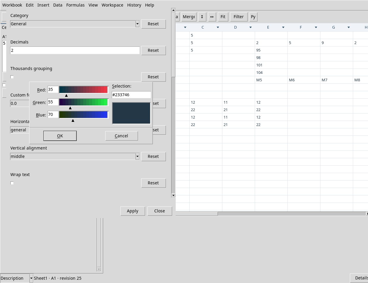
- Enter a color in the field or use Choose color…, adjust Red, Green and Blue, or enter the hexadecimal code in Selection and press Enter to confirm it. Press OK to adopt the color. Cancel exits the selector without applying it. The same choice is available for the border. Choose a family among the installed ones, such as DejaVu Sans Mono, and set a size of 6–72. The view starts at 13 with text color
#233746and white background. - Bold, Italic, Underline
- Independent checkboxes for bold, italic and underline.
- Border color, Border width (px), Border style, Borders
- Set the color, a width of 0–12 px and the style
solid,dashedordotted. In Borders choosenone,all,outer,inner,top,bottom,leftorrightaccording to the sides to cover.
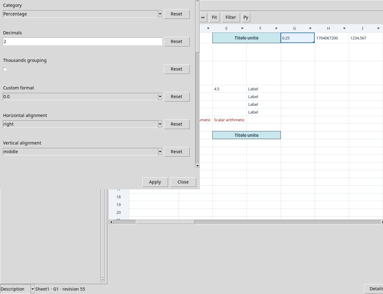
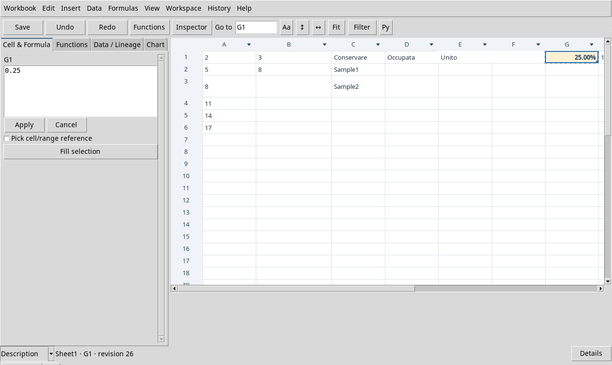
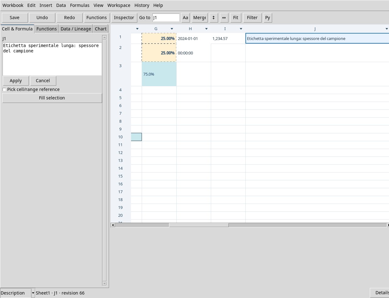
Try Percentage with two decimals on G1. The grid shows 25.00% and the inspector keeps 0.25. On I1, Number with two decimals and grouping shows 1,234.57 for 1234.567. Undo and Redo step through the style changes. Use Close to return to the grid after Apply. For date and time, use Unix seconds in UTC with s units or with no declared unit.
Merge, edit and split cells
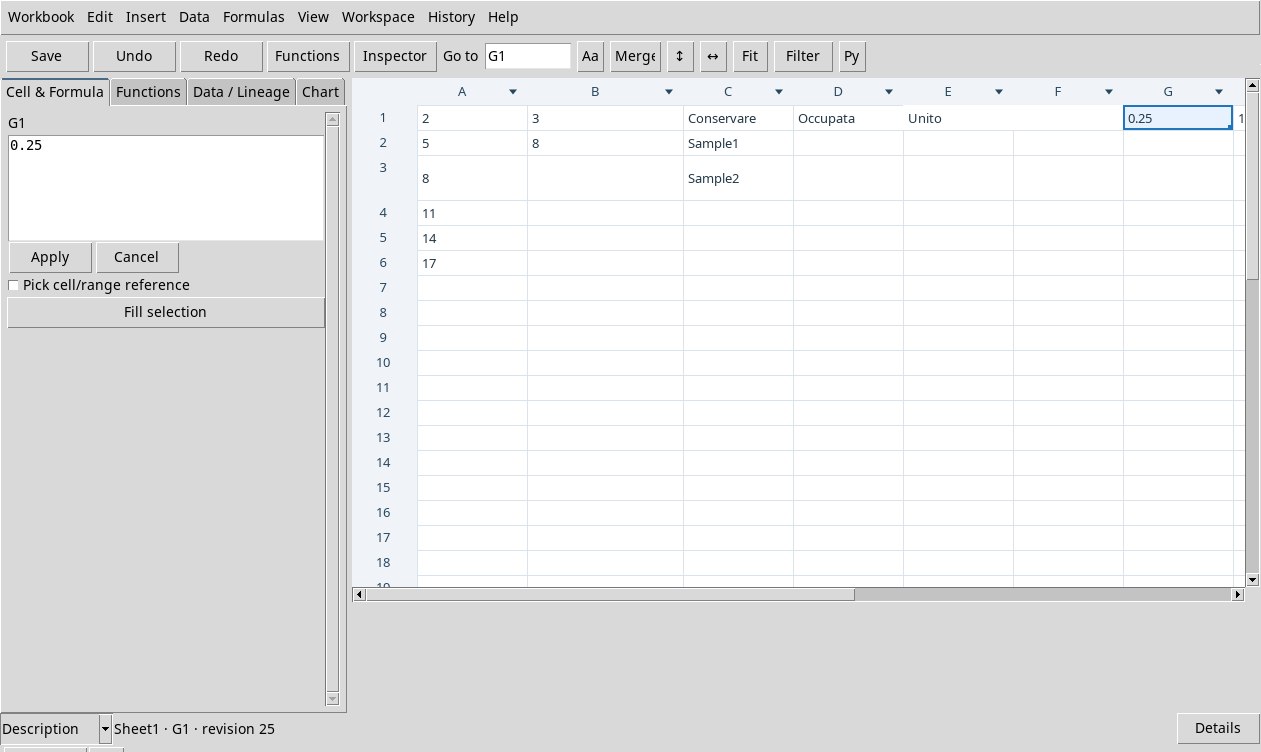
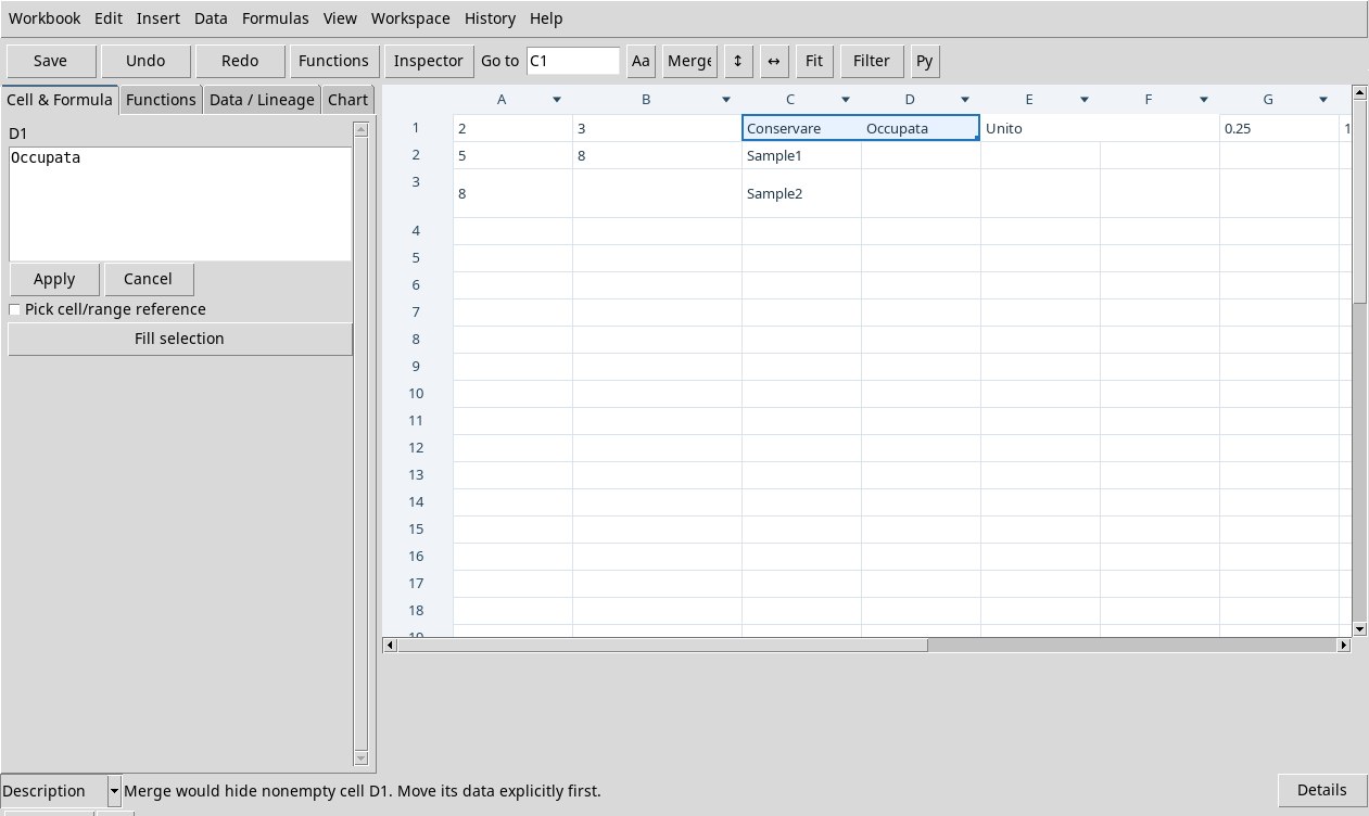
- Try Edit → Merge on C1:D1 when both cells are filled. The message indicates that the content of D1 would be hidden and asks you to move it explicitly. Keep both values, then use a free rectangle such as E1:F1.
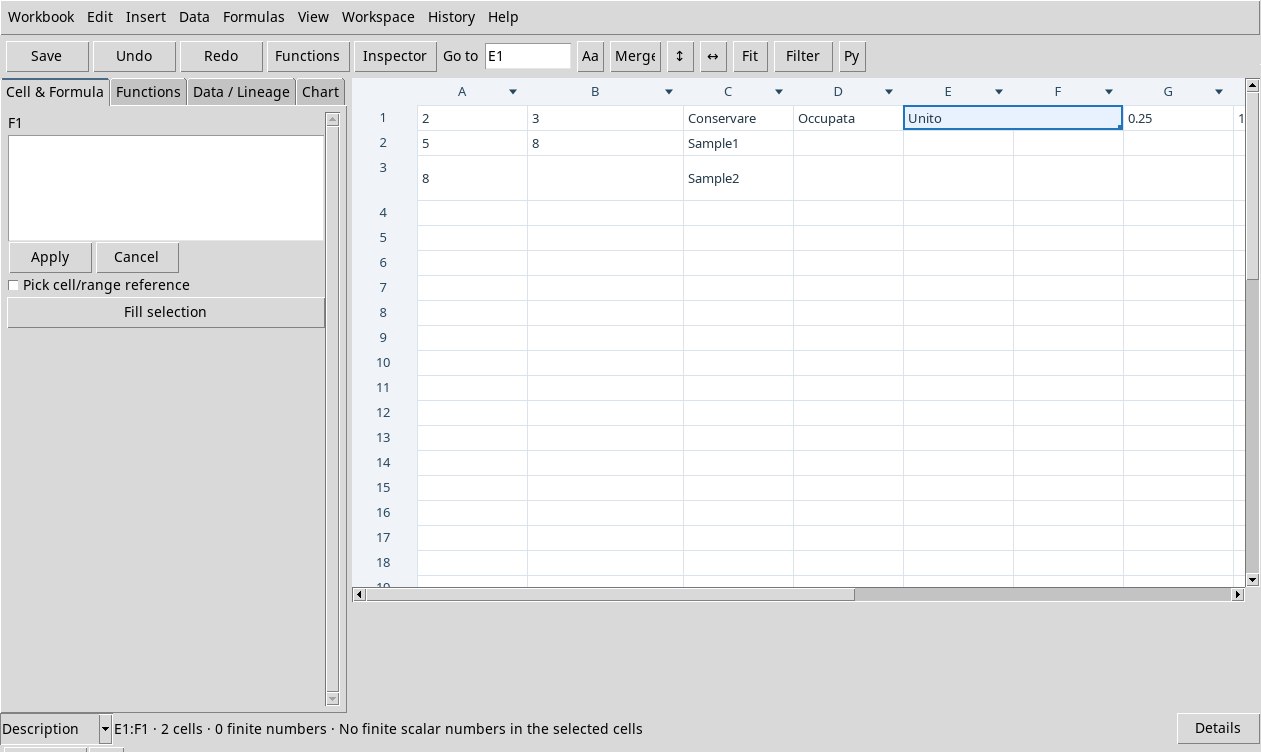
- Select E1:F1 with
Unitoin E1 and F1 empty. Use Merge. The data anchor is E1, at the top left. To change the label, select E1 explicitly and use Cell & Formula. To format the anchor choose Format Cells and adjust alignment and color. - Select the entire range E1:F1 and use Edit → Unmerge or Split in the context menu. E1 keeps the edited label and F1 becomes available again as an empty cell. With Undo you return to the merged region, with Redo you return to the separate grid. On a single ordinary cell Merge and Unmerge are disabled.
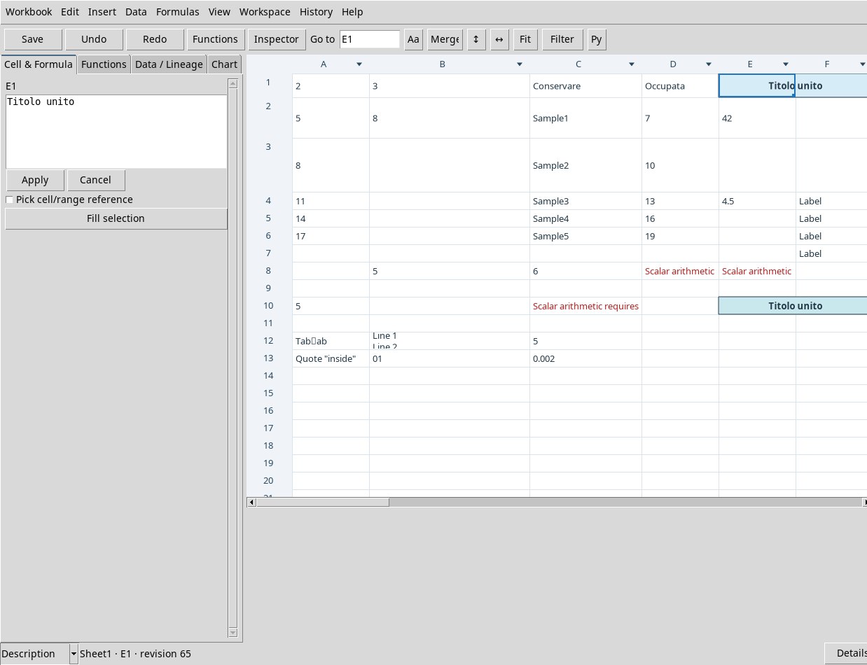
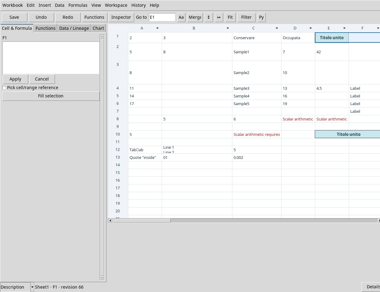
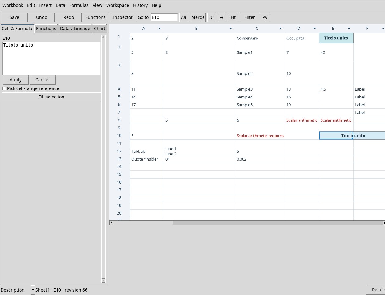
To copy the merge, select the whole E1:F1, then use Copy and paste into E10. The typed clipboard transfers the label, the style of E1 and the E10:F10 merge. Trying on F1 alone asks you to copy the whole range or to split it.
Adjust row heights and column widths
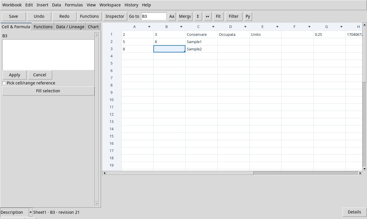
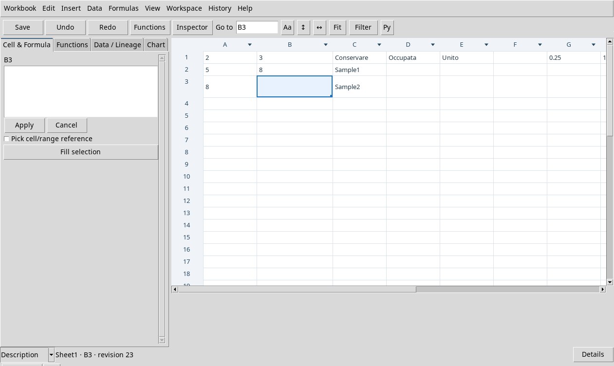
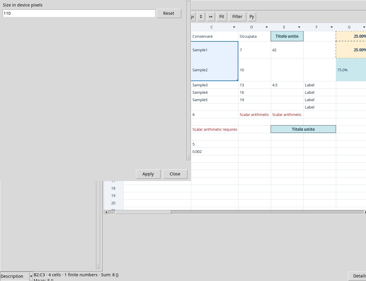
- Select B2:C3. Open Edit → Column width or the ↔ button. In Size in device pixels enter 185 and press Apply. You will get 185 px for B and C. Open Row height or ↕ and apply 58 px to rows 2 and 3. The allowed ranges are 35–2,000 for width and 16–2,000 for height.
- Alternatively, point to the right divider of the B header and drag it to the right. The column widens and the following ones shift. For row 3, drag down the divider below the number 3. Undo and Redo step through one gesture at a time.
- With a long text in J1 choose Edit → Auto-fit or Fit. The Viewer measures the selected occupied cells, taking into account font, text lines, rotation and wrapping. The interface also offers a double click on the header. If clicking the divider starts a manual resize, use Fit to apply the adjustment explicitly. Check the row after enabling wrapping.
Undo and saving your work
During the test, use Undo and Redo to check insertions, resizing, merges, formatting and clipboard operations. Distinguish the state of the open Workbook from the identity of the published resources. In the verified patch, defect 108 prevents saving changes to the Worksheet. The pre-registered template allows Jobs and publications, and a published Dataset can be consulted in the Session regardless of the open sheet. To save an exercise table outside the Worksheet, use Publish Dataset when its schema and units are suitable.