Native charts and publication
Create native charts from cells or Datasets, configure axes and units, and publish and reopen charts in GX-TXT.
Create a native chart from the grid
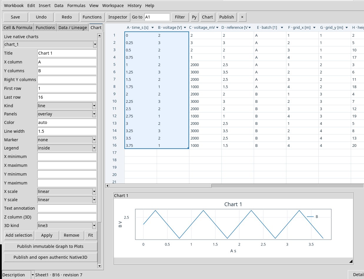
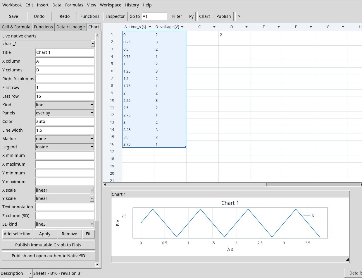
Take the data from the lab and bind time_s and voltage in A:B. Select A1:B16, then Insert → Native chart from selection or Chart → Add selection. The left column is X and the others are Y. A single-column selection proposes the next column for Y. A single-row selection also proposes the following row. The chart starts with line, a range derived from the selection, linear axes and the title Chart 1 title.
The live chart is in the pane below the grid. Open the same editor with Data → Charts / Publish… or View → Chart properties. Select a figure with the menu in Chart or by clicking the figure. Drag the title bar to move it and the handle at the bottom right to resize it. The wheel zooms, the middle button pans and a double click refits the view, like Fit. Remove removes the selected figure from the sheet.
Set source, panels and style
- Title, X column, Y columns, Right Y columns
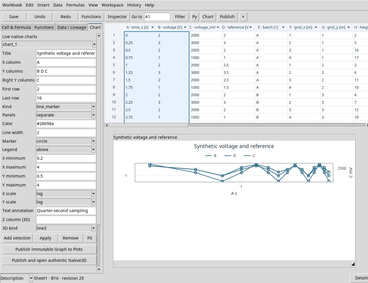
- Give a title and use coordinates from A to ZZ. List the Y columns separated by spaces, for example
B D C. WriteCin Right Y columns to send it to the right axis. Columns on the same axis must have compatible units. The right axis or separate panels allow independent scales. - First row, Last row
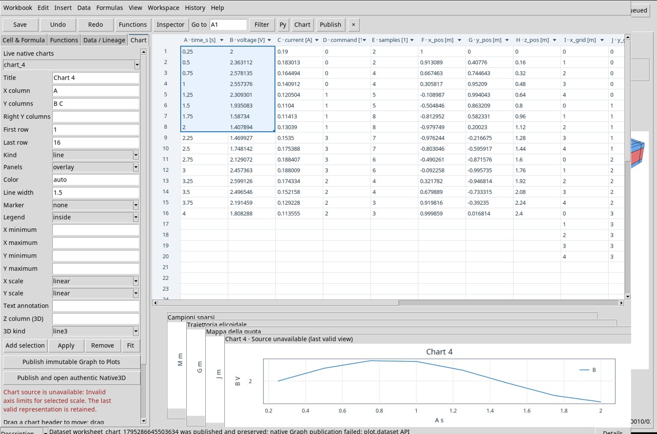
- Sets the inclusive window. The chart detaches its reference from the sheet it was created from. Limit the range to 20,000 rows and use columns that are internally homogeneous in units.
- Kind
linejoins points,scattershows points,line_markerjoins them and highlights them,stepuses steps andbarbars.- Panels
overlayoverlays the series to compare them in the same panel.separateseparates the series into panels. Check the units, scales and axis of each series.- Color, Line width
autochooses the default color of the context. You can specify#RRGGBB, for example#28698a. The width starts at 1.5 and must be positive.- Marker
noneleaves the style without a symbol. Choosecircle,square,triangle_up,triangle_down,diamond,plus,xorstarto distinguish the points. Check the type of representation when you want to see them.- Legend
nonehides it,insideshows it inside the area,above,below,left,rightplace it on the chosen side.- X minimum, X maximum, Y minimum, Y maximum
- Explicit limits for X and the left Y. Use a minimum smaller than the maximum. Leave the fields empty for automatic fitting. The unit is the one displayed on the axis.
- X scale, Y scale
- Use
linearfor uniform increments andlogfor factors. Limits and values shown on a logarithmic scale must be positive. The exercise times start at 0.25 s. Try a logarithmic X with minimum 0.1 s and maximum 5 s. - Text annotation, Apply
- Write an annotation to explain the view and press Apply to make the properties take effect. If the request is refused, read the status and correct the parameter indicated.
Freeze a chart in the Session
With a registered Workspace and the selected chart press Publish immutable Graph to Plots. The command creates a publication Dataset and records a Graph variant. Read the Dataset ID and the variant ID in the receipt. Open Plots in the main window for the persistent figure. Changing the cell later can change the live chart. The published Dataset and chart keep the data as they were at publication.
Import the four lab Datasets
- Open an empty Session. In Datasets open the Actions menu, then Import Dataset ZIP…. Select each ZIP and confirm with Import. The variable names and units can be read in the import summary.
- Open the Worksheet and import the Workspace template, giving it a name. Open that Workspace. In the empty template, repeat Data → Bind Dataset… for each row of the table below. Select all listed variables, set Destination start column according to the table, First Worksheet row to 1 and apply.
- Select A1:B8 as a starting point and create a figure. In the exercises you can reuse the same figure. Each new publication receives its own variant and keeps the table of that publication.
| Canonical Dataset | Start | Columns after binding | Rows |
|---|---|---|---|
| 2D time series | A | A time in s, B voltage in V, C current in A, D dimensionless command, E dimensionless count | 1–16 |
| Helix | F | F, G, H: X, Y, Z coordinates in m | 1–16 |
| Elevation on a Cartesian grid | I | I, J: X, Y coordinates in m; K: elevation Z in m | 1–20 |
| Irregular samples | L | L, M: X, Y coordinates in m; N: elevation Z in m | 1–14 |
The sequences are synthetic. The time block has 16 time points spaced 0.25 s apart. The helix makes about one turn of radius 1 m with a vertical step of 0.16 m between samples. The grid contains all combinations of five X and four Y values. The cloud uses 14 irregular coordinates, each with an elevation.
Configure and publish a three-dimensional chart
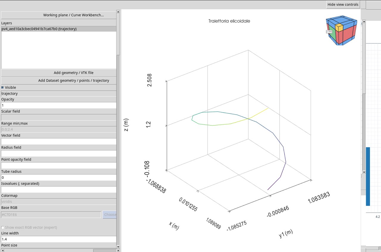
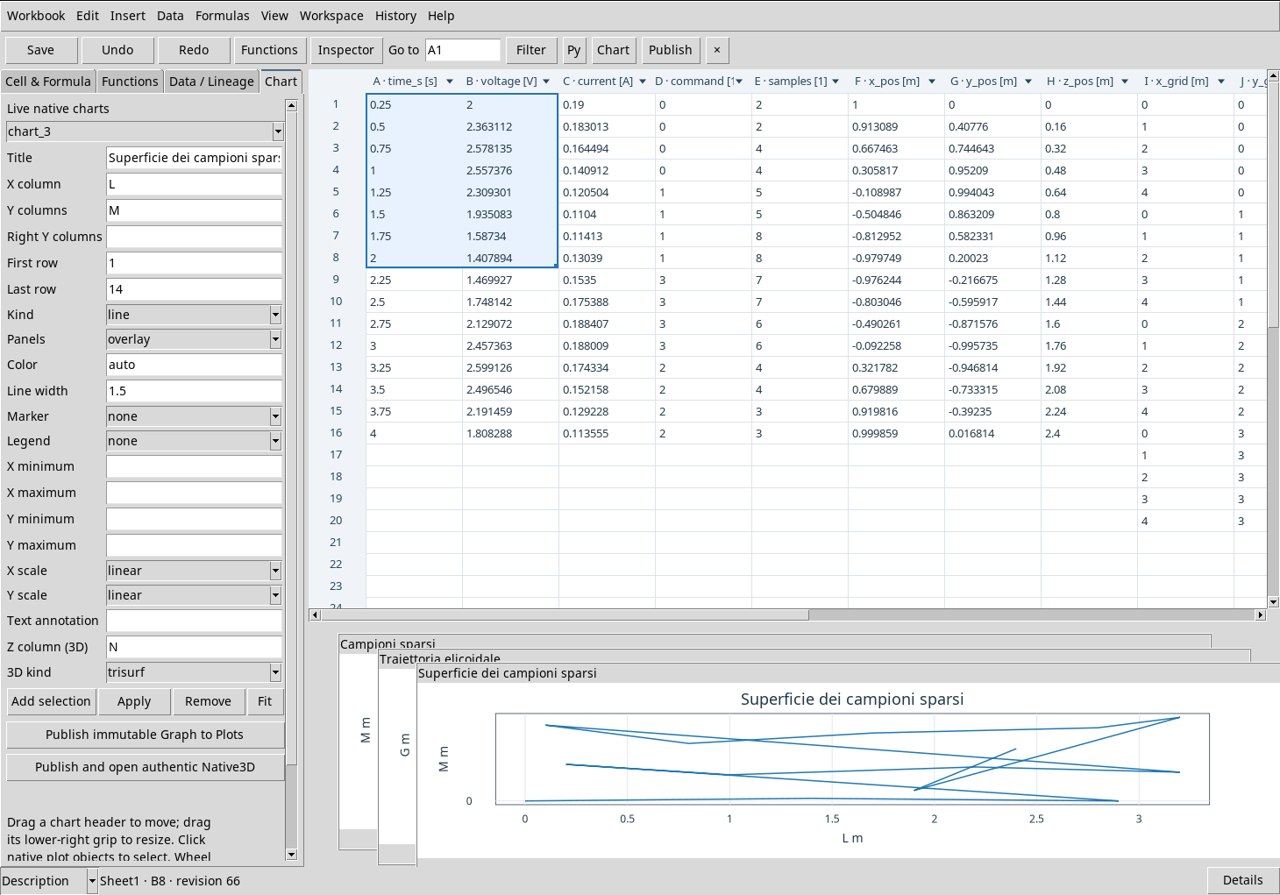
Set X column, the first column in Y columns, Z column (3D), the title, and the row range. Choose 3D kind and click Apply. In the Worksheet pane the figure follows the 2D view settings. For the XYZ representation use Publish and open authentic Native3D. The published Dataset includes x, the y1 columns and so on, and z. The 3D chart uses X, y1, and Z. Style properties from the 2D panel apply to the 2D view. Adjust the viewpoint in the Native3D Viewer.
With Z empty, the command asks you to choose a column. Read the publication variant before moving to Plots. The grid exercises use all the X, Y pairs of the rectangle. In the view, the elevation or its color is associated with the pair in the same row.
Reopen a chart and recognize the published resource
- Apply updates the live figure. Publish immutable Graph to Plots produces the XY Graph. Publish and open authentic Native3D produces the XYZ Graph and opens the interactive view.
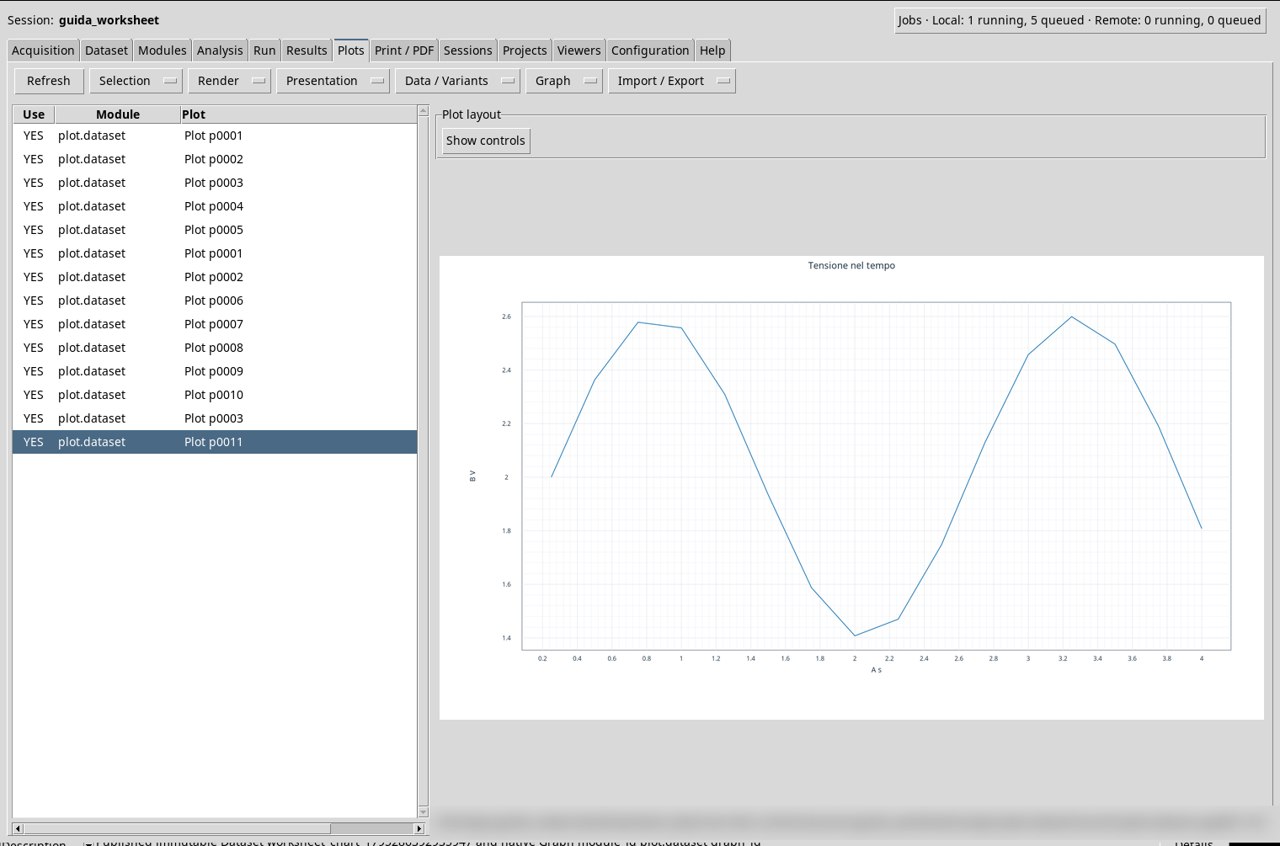
- Go back to the main window and open Plots. Use Refresh if necessary. Select the Plot pNNNN row indicated in the receipt. The Module column shows
plot.dataset. To distinguish two variants with the same number, check XYZ or XY in the row information and the title in the figure. - Click Graph → Open PNG 1:1 to open the image at its original size. The result screenshots of the exercises were obtained from this menu. The charts remain accessible with the Worksheet closed. In testing, the 12 Graphs were still present after restarting GX-TXT and reopening the original Session. When you use another Session, import the exercise Datasets and publish again to get the Graphs in that Session.
Publish only the Dataset
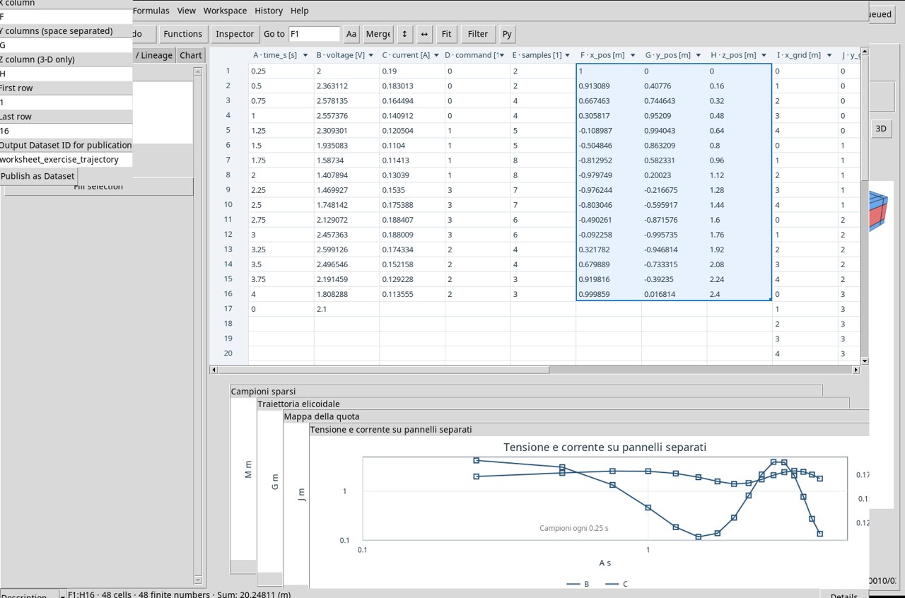
To freeze the measurements in a table, use Data → Publish Dataset…. Set X column to F, Y columns (space separated) to G, Z column (3-D only) to H and rows 1–16. In Output Dataset ID for publication write worksheet_exercise_trajectory, then press Publish as Dataset. The published table exposes x, y1 and z, each with 16 rows and in m. The Dataset appears in Datasets. A Graph variant requires one of the publishing buttons of the Chart tab.
Correct sources, values and units
- With an empty range the Viewer reports that there are no finite pairs. Reopen Chart and choose two columns with measurements paired by row.
- A logarithmic scale requires positive limits. Check the samples that fall outside the domain. Set a window of entirely positive samples, or use a linear scale when zero is a meaningful value.
- For two series with different dimensions, such as V and A, use Right Y columns or
separate. Check that each axis displays its own unit. - Check that First row precedes or coincides with Last row, that the minimum and maximum limits are increasing, that Line width is positive and that a specific color has the form
#RRGGBBshape.
If incompatible limits leave the message Source unavailable (last valid view) displayed, the pane keeps the last valid representation. Correct the limits or clear them and apply again. A failed publication can report Dataset … was published and preserved. The Dataset is then already in the Session, and Plots must be checked separately for any Graph.
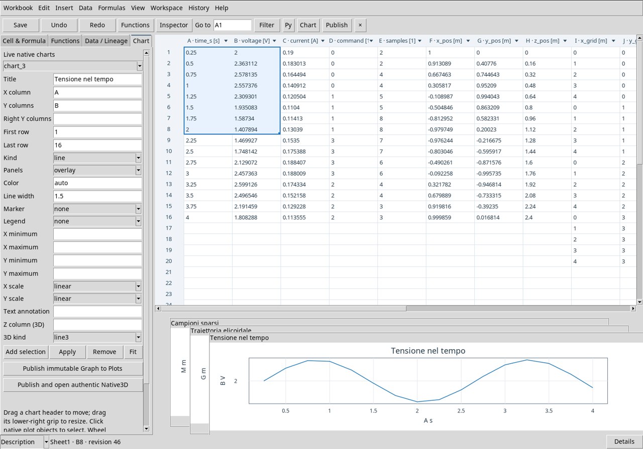
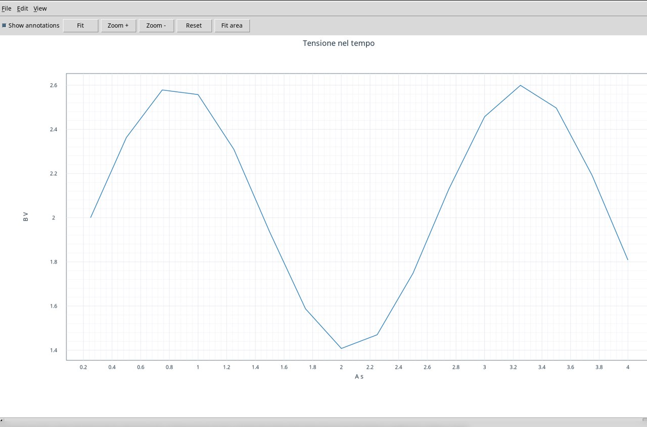
Voltage line · line
Use the already associated exercise Dataset. In Chart set X column A, Y columns B and Kind line. Set First row to 1 and Last row to 16. Leave Marker set to none. Read the X axis in s and the Y axis in V. The segments follow the voltage samples in order and let you recognize the periodic variation. The available values correspond to the acquired time points. Press Apply and Publish immutable Graph to Plots.
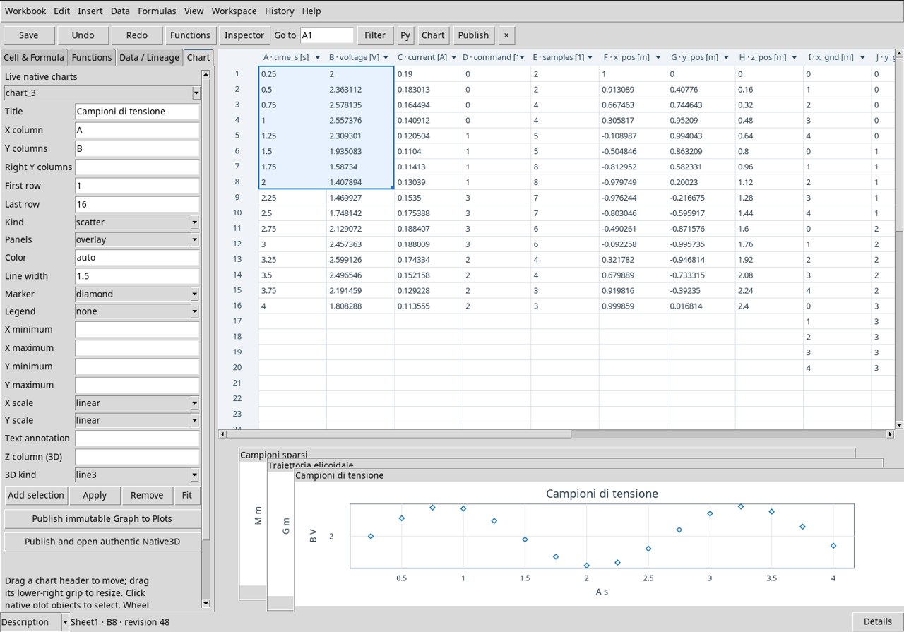
Scatter of voltage samples · scatter
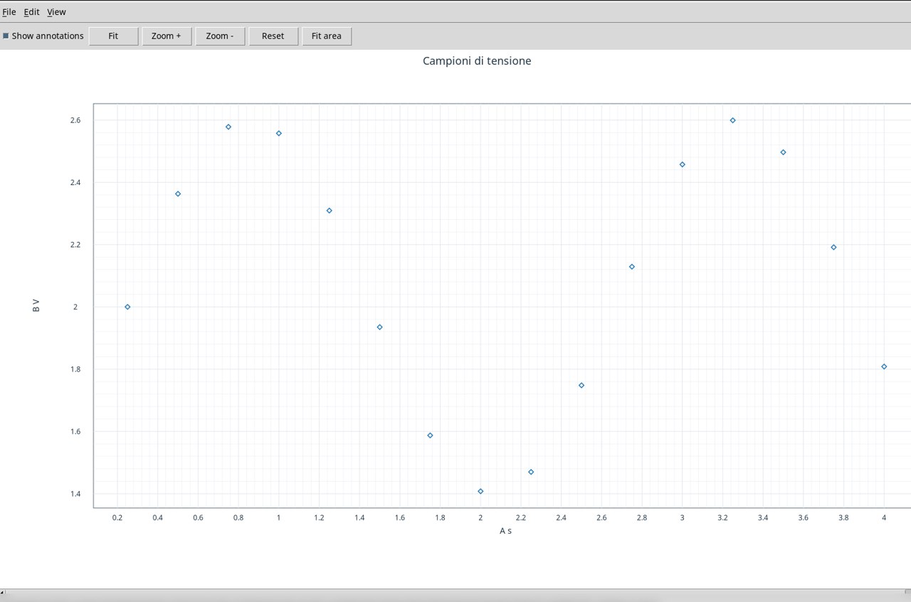
Use the already associated exercise Dataset. In Chart set X column A, Y columns B and Kind scatter. Set First row to 1 and Last row to 16. Set Marker to diamond. Each diamond marks a time–voltage pair. Check the horizontal spacing of 0.25 s between points and the vertical amplitude in V. Press Apply and Publish immutable Graph to Plots.
Voltage and current on two axes · line_marker
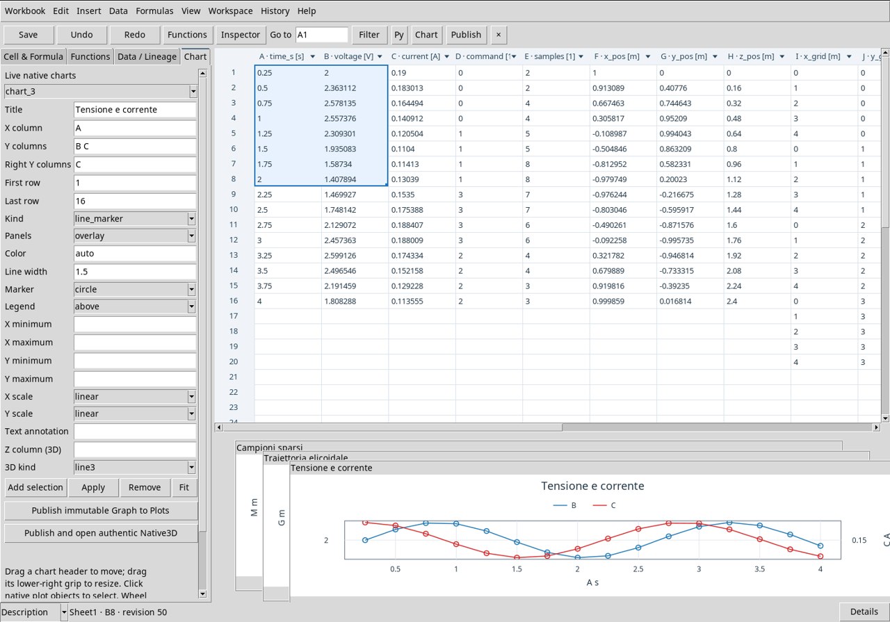
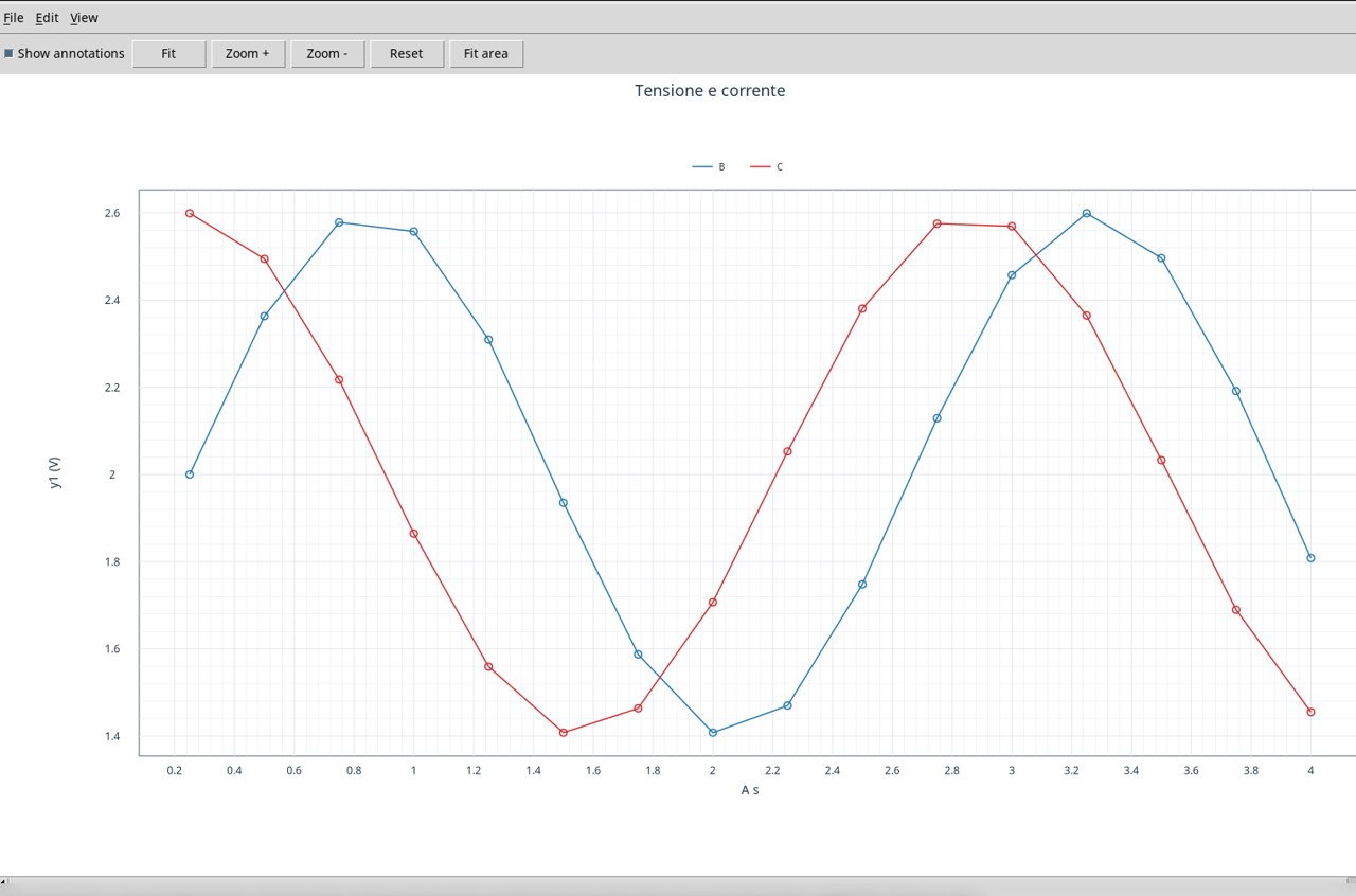
Use the already associated exercise Dataset. In Chart set X column A, Y columns B C and Kind line_marker. Set First row to 1 and Last row to 16. In Right Y columns write C. Choose Panels overlay, Marker circle and Legend above. Series B uses the left scale in V. Series C uses the right scale in A. Recognize the two trends from the legend and always read the unit on the corresponding side. Press Apply and Publish immutable Graph to Plots.
Step command · step
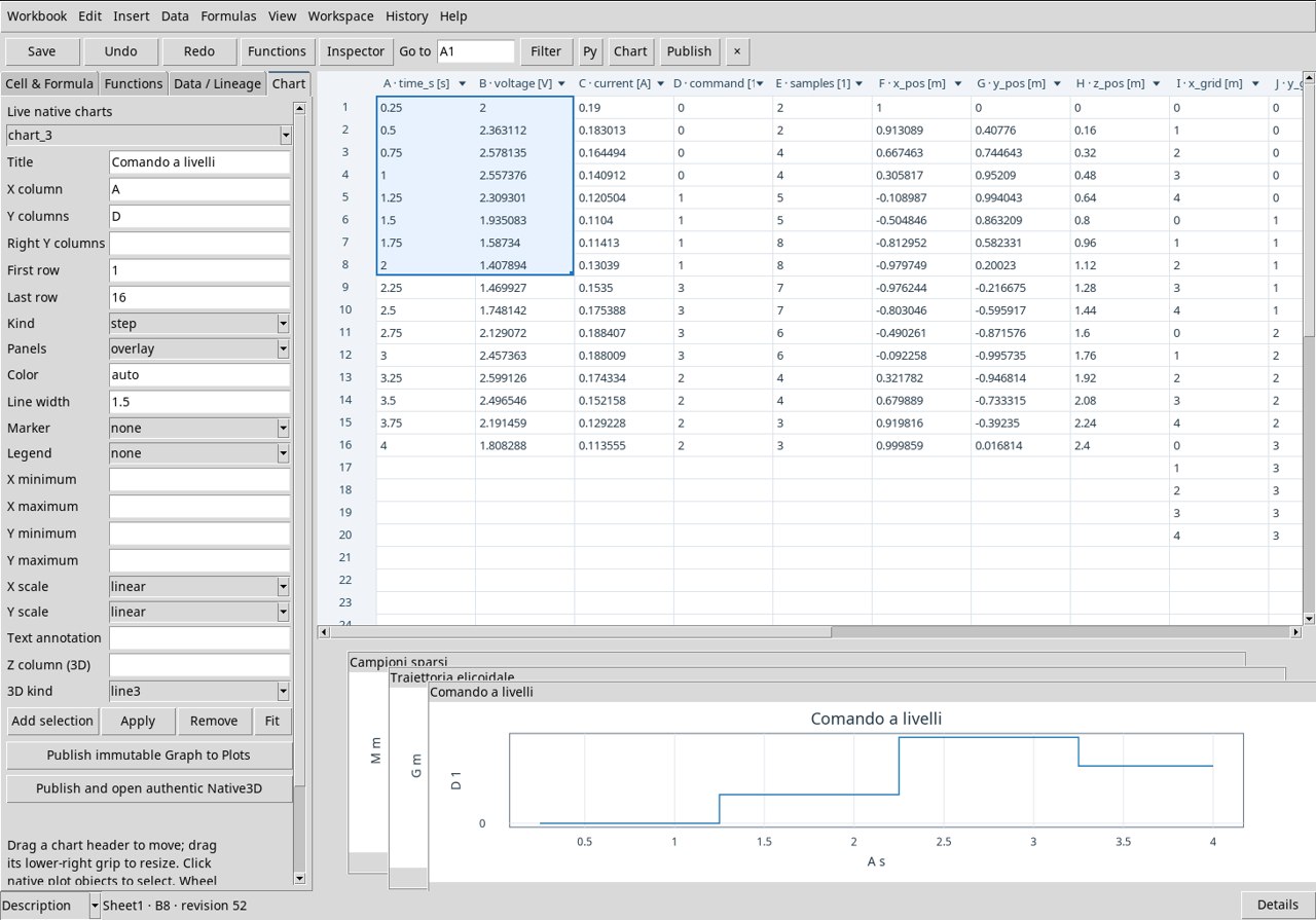
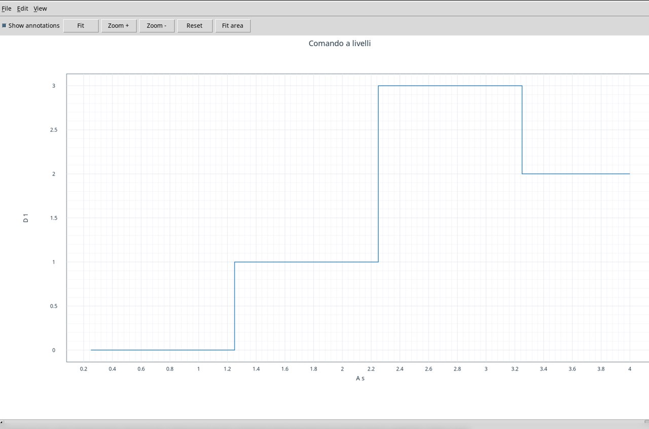
Use the already associated exercise Dataset. In Chart set X column A, Y columns D and Kind step. Set First row to 1 and Last row to 16. D contains four dimensionless command levels, 0, 1, 3, 2. Read the horizontal sections as levels held between samples, and the transitions as a function of time, in s. Press Apply and Publish immutable Graph to Plots.
Counts per time point · bar
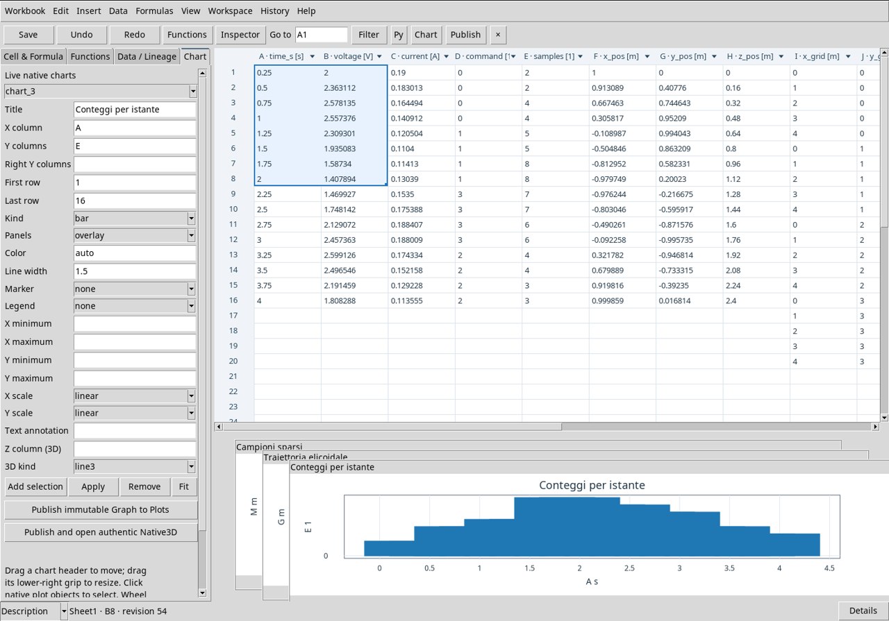
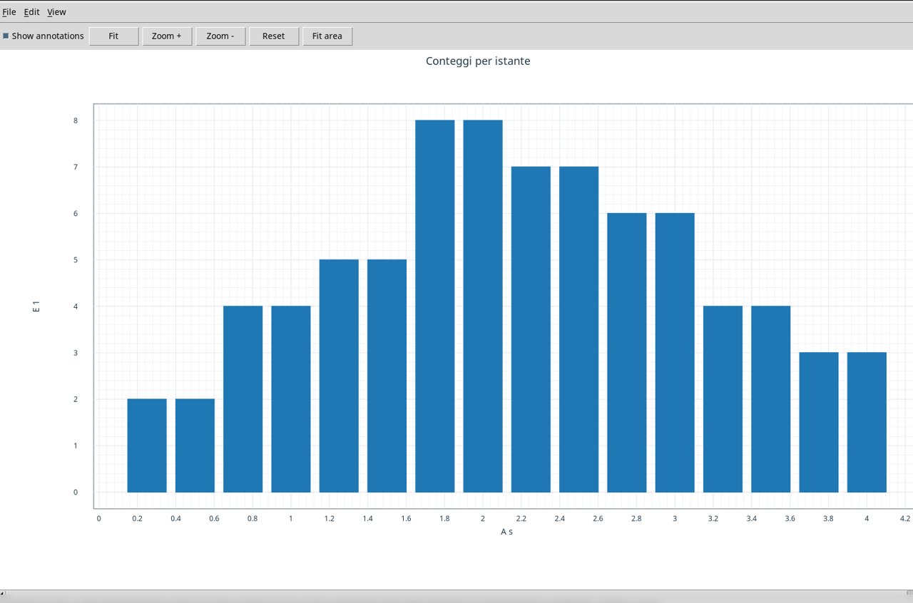
Use the already associated exercise Dataset. In Chart set X column A, Y columns E and Kind bar. Set First row to 1 and Last row to 16. Each bar is placed at its time point, in s. The height shows the count of the same row. The two consecutive maxima are equal to 8. Press Apply and Publish immutable Graph to Plots.
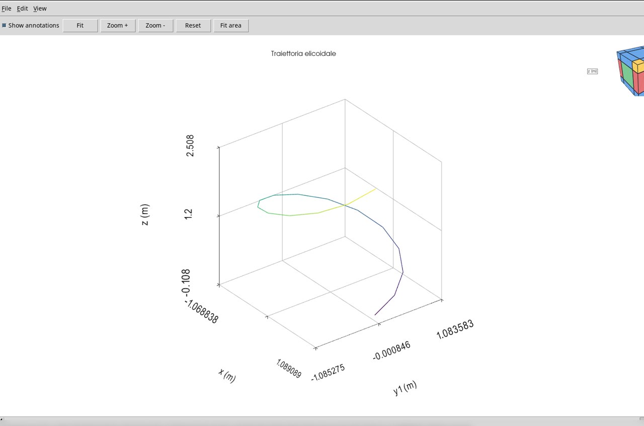
Helical trajectory · line3
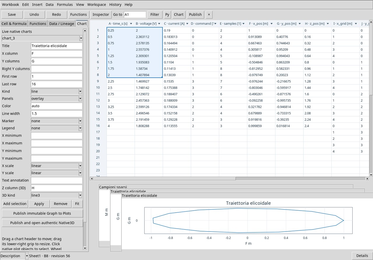
Use the already associated exercise Dataset. In Chart set X column F, Y columns G, Z column (3D) H and 3D kind line3. Set First row to 1 and Last row to 16. The segments connect the samples in row order. Check that X and Y vary between −1 and 1 m and that Z grows from 0 to 2.4 m. Rotate the view to distinguish vertical displacement and rotation. Press Apply and Publish and open authentic Native3D.
Irregular samples in space · scatter3
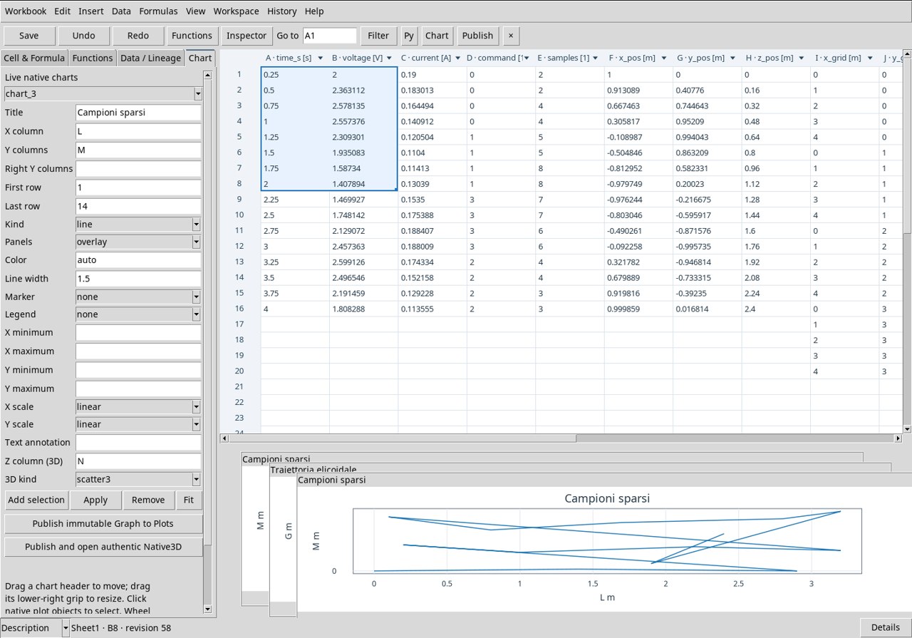
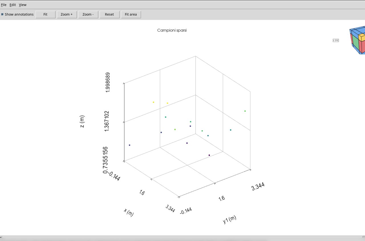
Use the already associated exercise Dataset. In Chart set X column L, Y columns M, Z column (3D) N and 3D kind scatter3. Set First row to 1 and Last row to 14. Each point keeps the three coordinates in m of its row. Rotate the view to recognize the distribution in the XY plane and the different elevations. The spacing between samples changes from one position to another. Press Apply and Publish and open authentic Native3D.
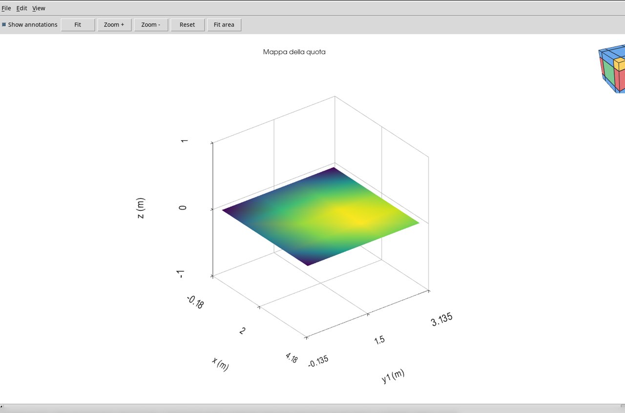
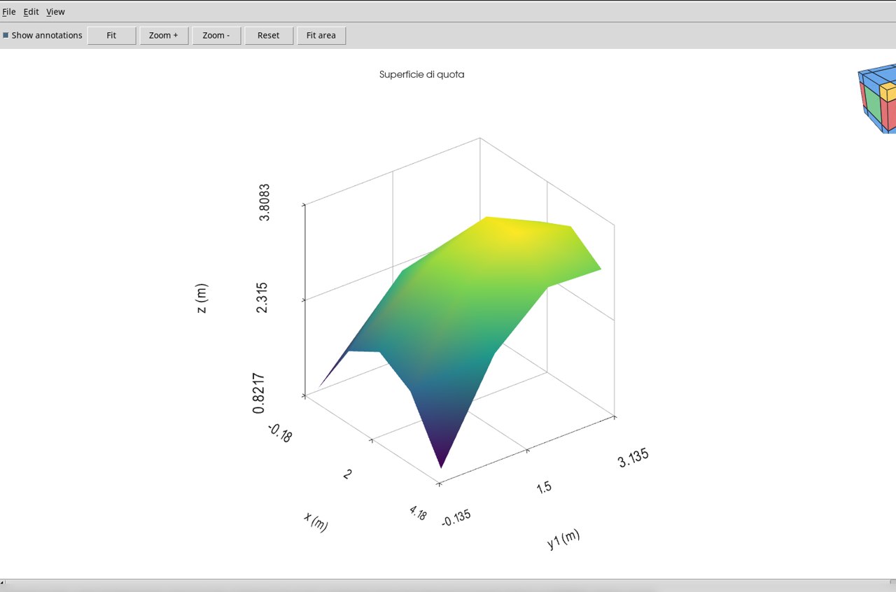
Elevation surface · surface
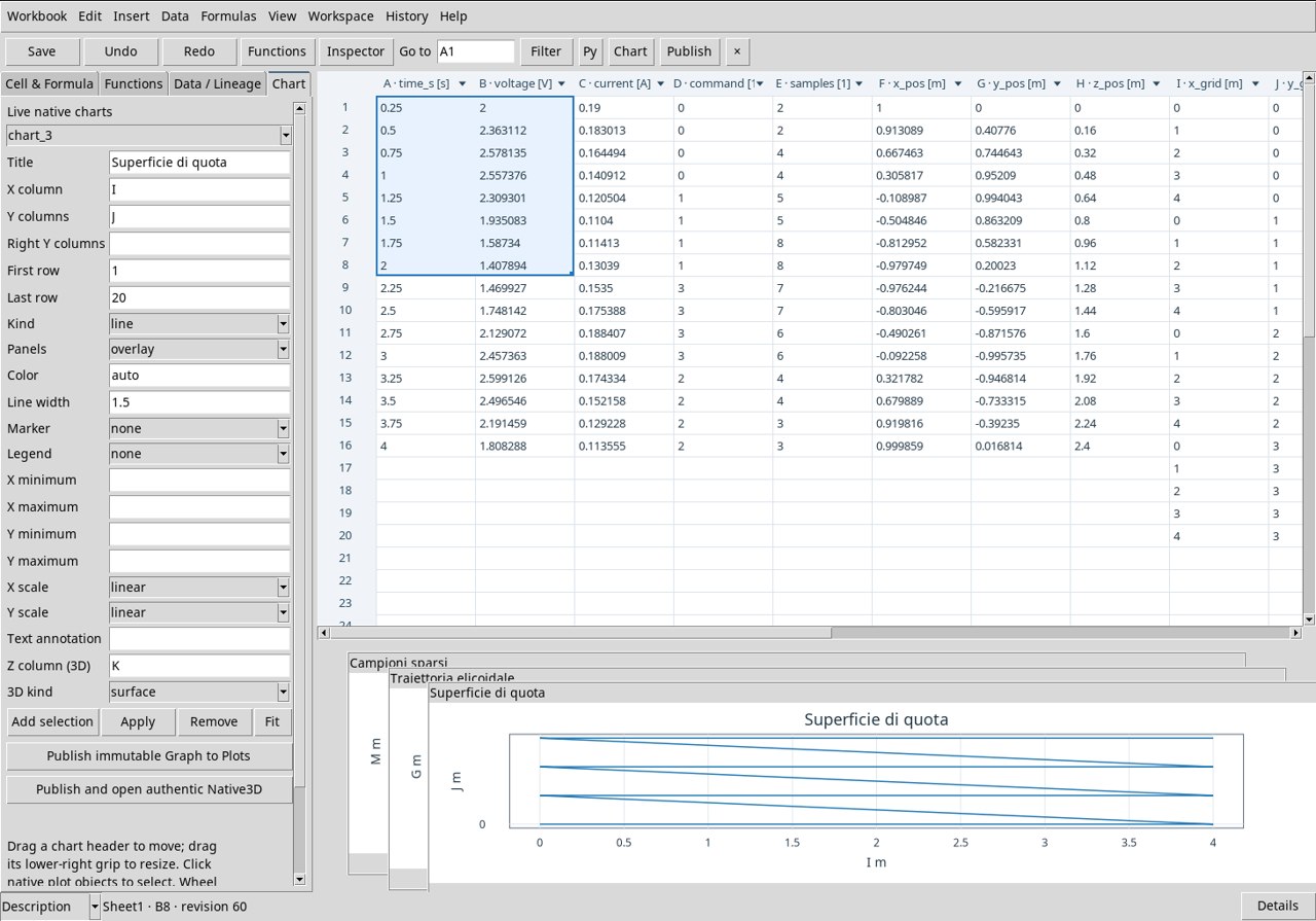
Use the already associated exercise Dataset. In Chart set X column I, Y columns J, Z column (3D) K and 3D kind surface. Set First row to 1 and Last row to 20. The colored surface represents Z in m on the 5 × 4 grid. Identify the highest area and compare it with the elevations measured in the neighboring rows. Press Apply and Publish and open authentic Native3D.
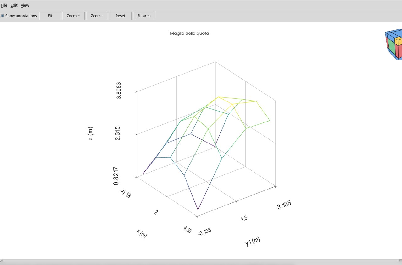
Elevation mesh · mesh
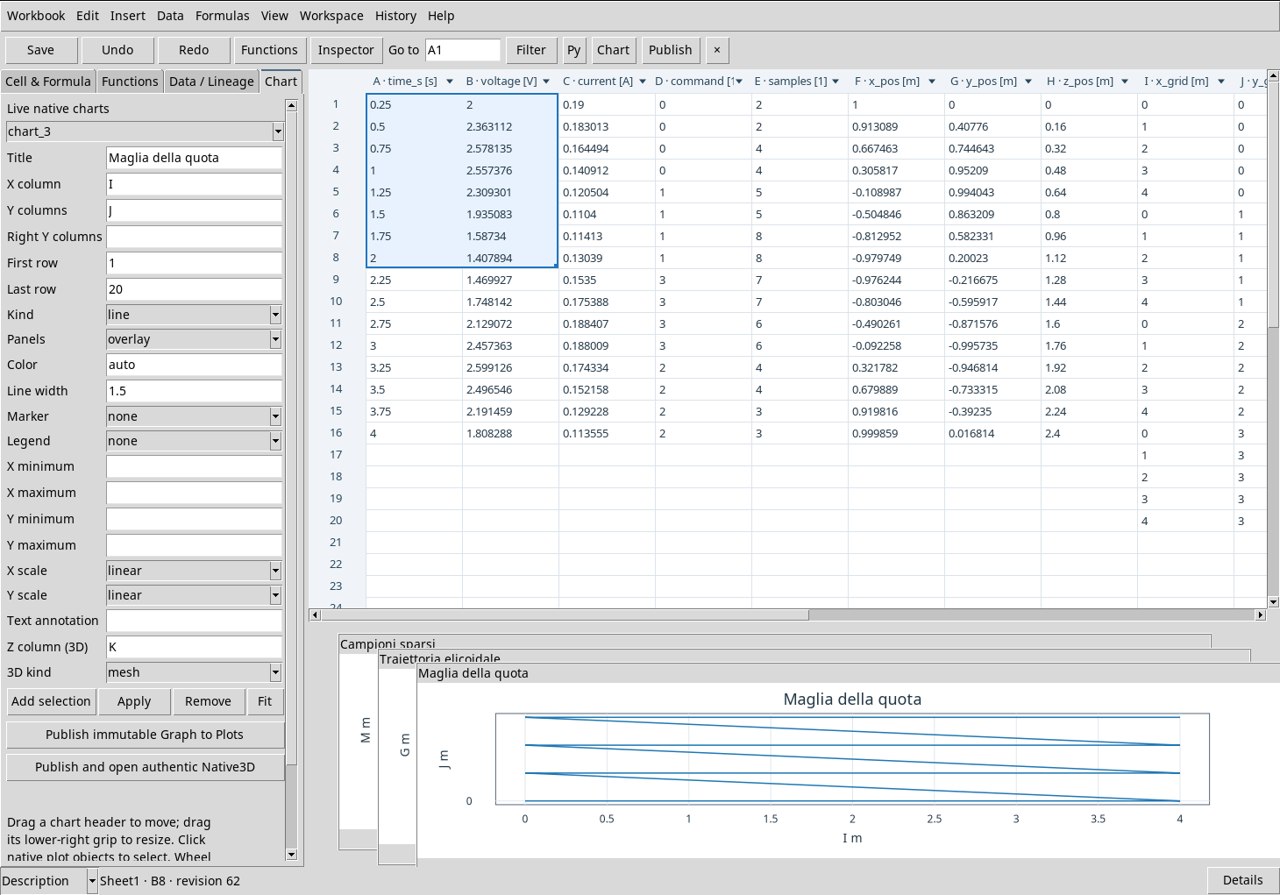
Use the already associated exercise Dataset. In Chart set X column I, Y columns J, Z column (3D) K and 3D kind mesh. Set First row to 1 and Last row to 20. The lines show the structure of the grid. Follow an alignment at constant X or Y to read how the elevation in m changes between adjacent positions. Press Apply and Publish and open authentic Native3D.
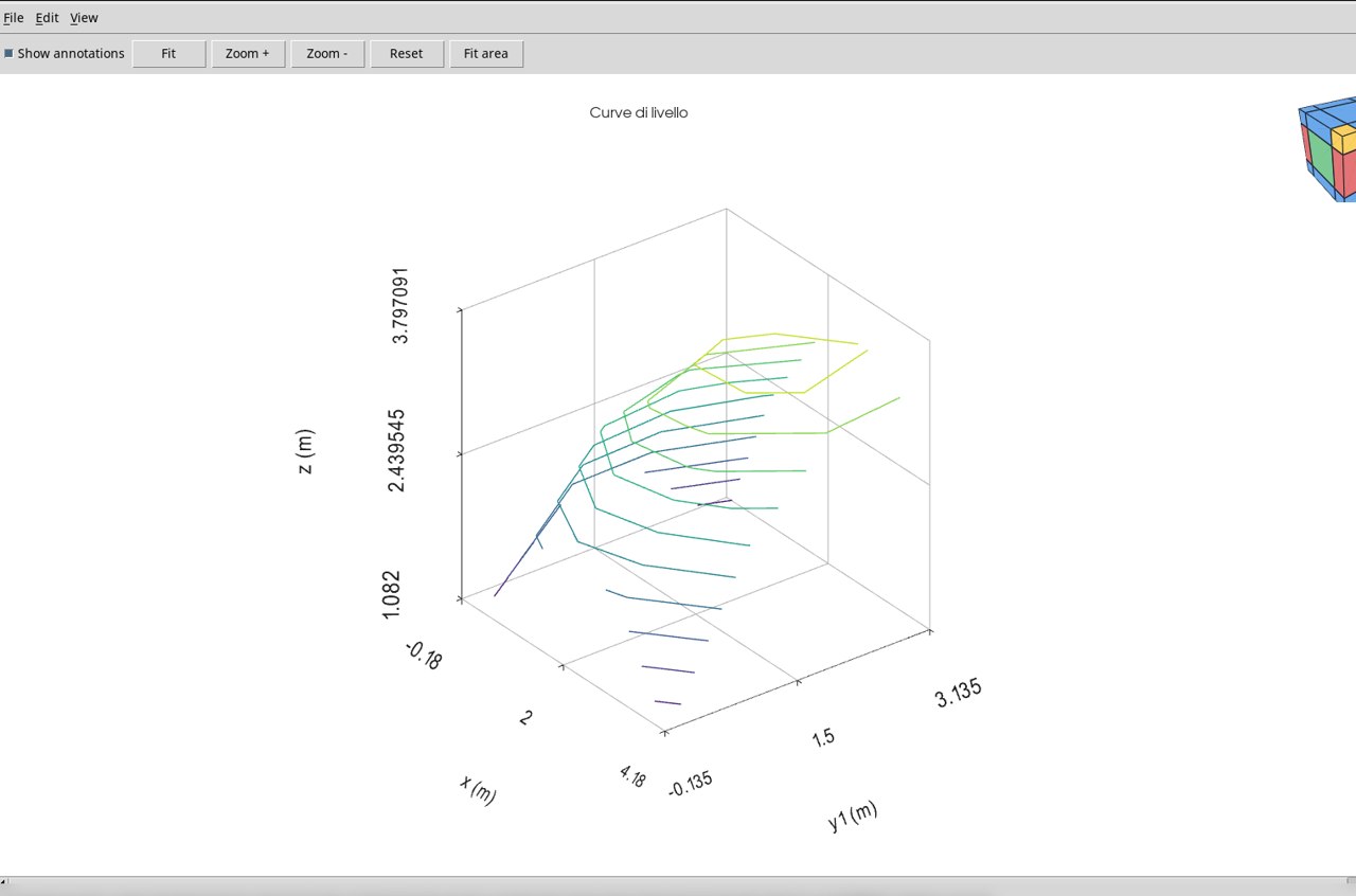
Elevation contour lines · contour3
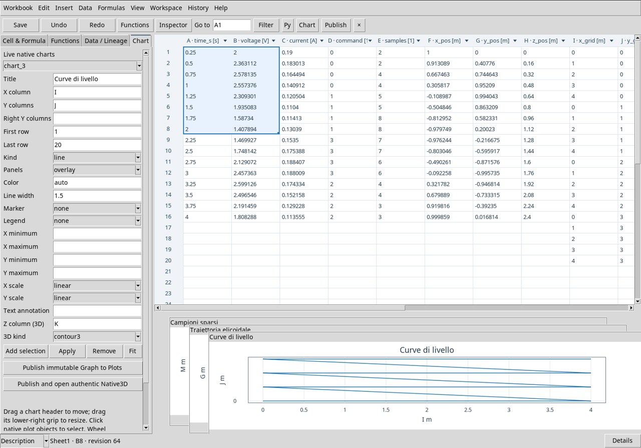
Use the already associated exercise Dataset. In Chart set X column I, Y columns J, Z column (3D) K and 3D kind contour3. Set First row to 1 and Last row to 20. Each curve represents one elevation value, obtained from the grid. Interpret level and position using the axes in m and the scale displayed by the Viewer. Press Apply and Publish and open authentic Native3D.
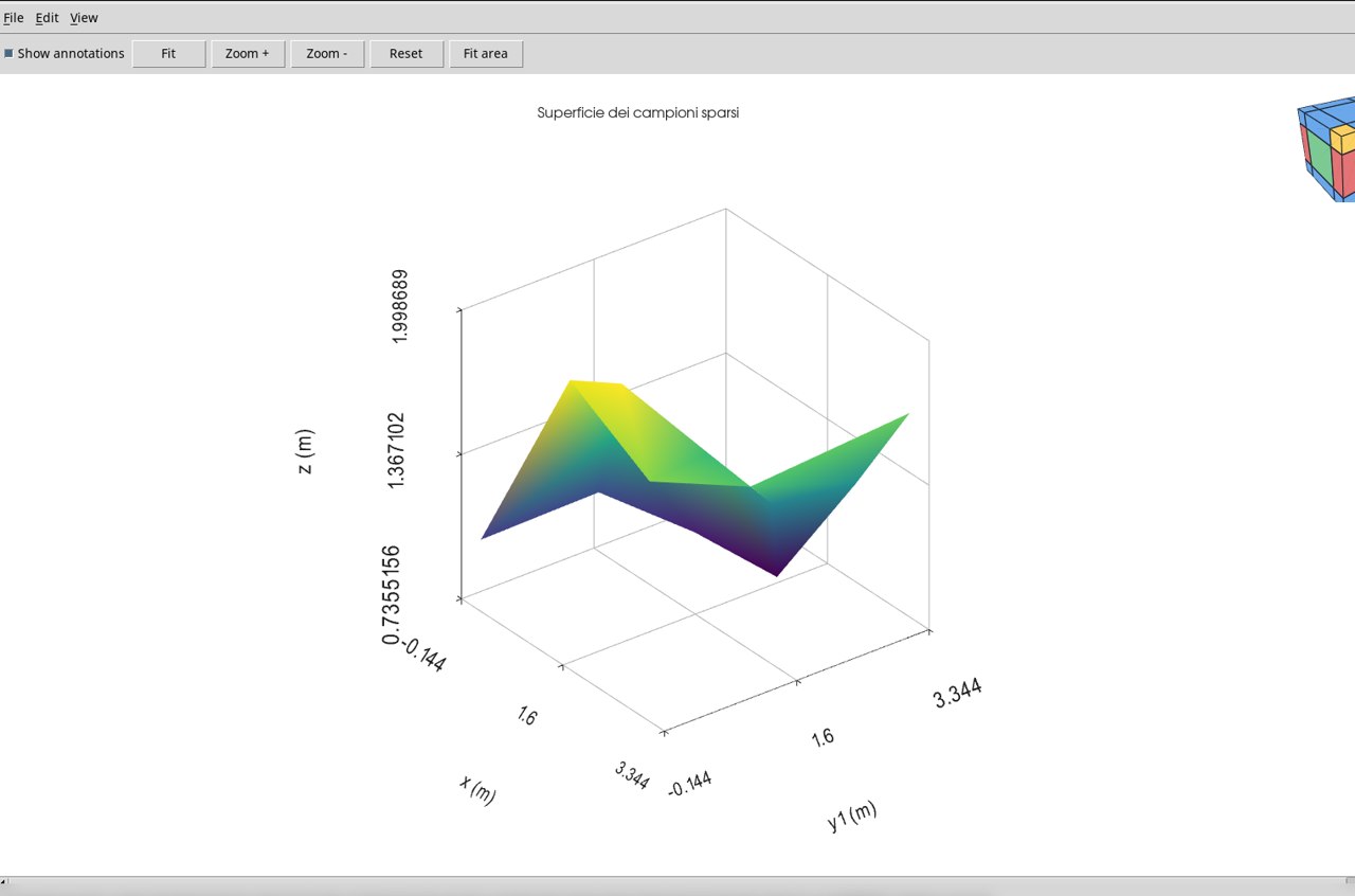
Triangulated surface from scattered points · trisurf
Use the already associated exercise Dataset. In Chart set X column L, Y columns M, Z column (3D) N and 3D kind trisurf. Set First row to 1 and Last row to 14. The samples in the XY plane define the triangles. The measured elevations are at the vertices. The face between vertices makes the local connection visible and must be interpreted according to the actual density of the samples. Press Apply and Publish and open authentic Native3D.
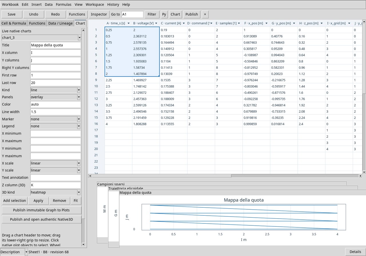
Elevation color map · heatmap
Use the already associated exercise Dataset. In Chart set X column I, Y columns J, Z column (3D) K and 3D kind heatmap. Set First row to 1 and Last row to 20. The position of the cell in the map uses X and Y. The color represents the elevation Z in m. Use the color scale to compare the position of the maximum and the lowest areas. Press Apply and Publish and open authentic Native3D.