

GX LII-2 – Experimental Characterization of the Measurement System
Where I am starting from
In the previous article I described the construction of the injection system and the first tests, initially performed on an LM358-based active circuit and later on several resistive networks of the calibration bench.
The measurements on the dividers revealed an interesting behavior. Reversing the transformer secondary connections produces two different responses, which I called measurement A and measurement B. Under some conditions, averaging the two measurements compensates for this asymmetry very effectively, while increasing the impedance of the test circuit leaves an error component that is not removed by the simple A/B average.
The case of the approximately 33 kΩ + 33 kΩ divider clearly showed this second behavior and left open the need to better understand which parameters affect the measurement.
To continue the characterization, I had decided to use a constant generator amplitude of 300 mVpp, in order to eliminate at least one variable when comparing different configurations.
However, the first subsequent measurements showed that this choice itself deserves experimental verification.
The injection-amplitude problem
The amplitude set on the generator does not necessarily match the amplitude of the signals subsequently measured on the two sides of the injection point.
Depending on the network impedance and frequency, VOUT and VSENSE can become very small. This phenomenon was already visible with the 33 kΩ + 33 kΩ divider and becomes even more evident with the lower-impedance divider, approximately 3.3 kΩ + 3.3 kΩ.
Keeping Vgen rigidly fixed at 300 mVpp may therefore not always be the best choice: a signal that is too small worsens the signal-to-noise ratio and makes it more difficult to obtain an accurate magnitude measurement and, above all, an accurate phase measurement.
The question therefore becomes:
is it really necessary to keep Vgen constant, or can I adapt its amplitude to the conditions of the circuit being measured?
How to verify whether Vgen can be varied
If the system operates in its linear region, changing the amplitude of the excitation signal should not change the measured transfer function.
I can therefore measure the same circuit using different Vgen values and compare the results. If magnitude and phase remain essentially unchanged while only the amplitude of the acquired signals increases, raising Vgen is not altering the behavior I want to measure.
There is, however, a second check that can be performed directly on the acquired data.
The GNU Octave script I use to process the oscilloscope CSV files does not only fit the fundamental. It can also include the first harmonics and returns, for each channel, their levels, THD, and the fit residual.
This makes it possible to observe whether significant harmonic components begin to appear as Vgen is increased and therefore to experimentally identify the approach to a nonlinear operating condition.
The criterion I intend to use will therefore not simply be to obtain an apparently clean sine wave on the oscilloscope, but to verify simultaneously:
- stability of the measured magnitude;
- phase stability;
- harmonic behavior;
- THD;
- fit residual;
- actual amplitude of the VOUT and VSENSE fundamental components.
A small change to the setup
I decided to modify the trigger setup.
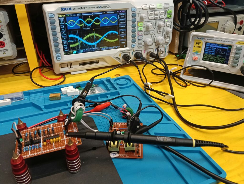
When the measured signals become very small, using one of them directly as the trigger source can make the horizontal display unstable. I therefore used the second channel of the function generator as a synchronized reference and connected it to oscilloscope CH3, using it exclusively as the trigger source.
CH1 and CH2 therefore remain dedicated to VSENSE and VOUT respectively, and the data processing does not change, while the waveforms are more stable on screen even when their amplitude is low.
Measurement results
For this comparison I used the acquisitions already made during the previous measurement session and today added the series on the 3.3 kΩ + 3.3 kΩ divider with Vgen fixed at 300 mVpp.
In today’s acquisitions, as mentioned, I used oscilloscope CH3 as the trigger source, driving it with the synchronized second channel of the function generator. With this configuration I used a memory depth of 300 kpts instead of 600 kpts. Despite the shorter acquisition window, the greater trigger stability made the signals much steadier and easier to read, especially under conditions where their amplitude is low.
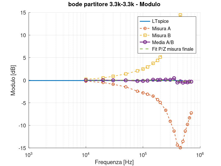
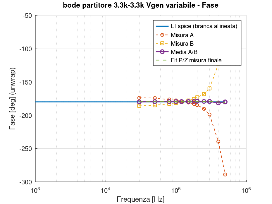
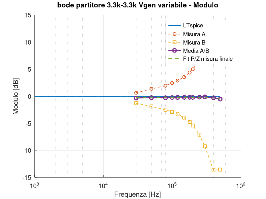
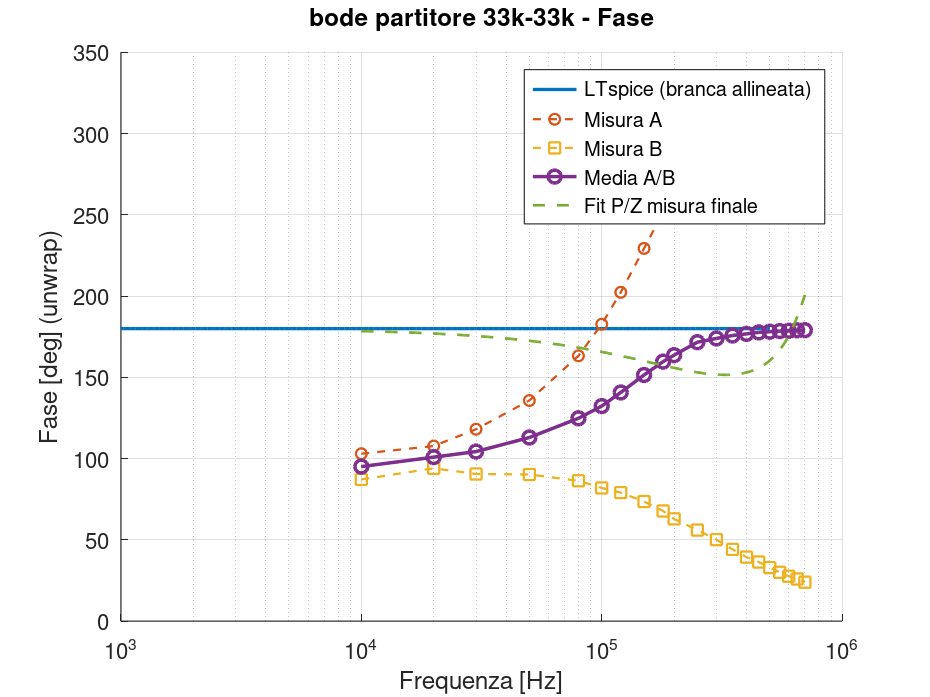
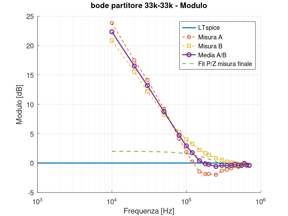
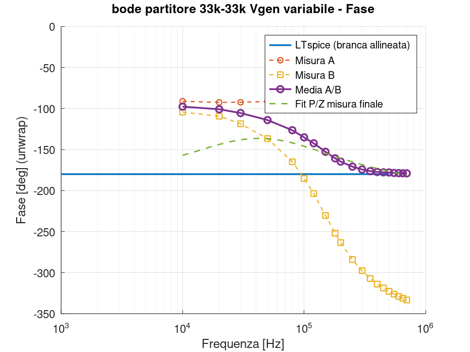
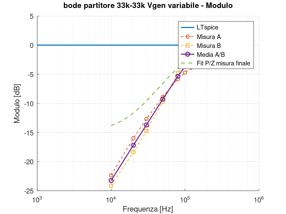
The following gallery collects the magnitude and phase plots for the available series, including measurements A and B, their average, and the LTspice reference.
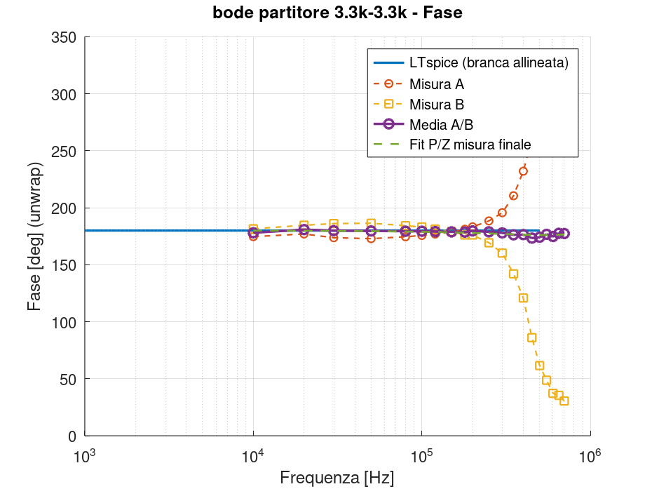 Partitore 3,3 kΩ + 3,3 kΩ – Vgen = 300 mVpp, fase. Confronto tra misura A, misura B, media A/B e riferimento LTspice.
Summary data
The following tables collect, for the two dividers, the Vgen values used and the parameters obtained from the harmonic analysis, directly comparing the acquisitions performed at 300 mVpp with those performed using variable Vgen.
3.3 kΩ – 3.3 kΩ divider
| f | Fixed Vgen | Fixed THD CH1 A/B ; CH2 A/B | Fixed H2 [dBc] CH1 A/B ; CH2 A/B | Fixed H3 [dBc] CH1 A/B ; CH2 A/B | Variable Vgen | Variable THD CH1 A/B ; CH2 A/B | Variable H2 [dBc] CH1 A/B ; CH2 A/B | Variable H3 [dBc] CH1 A/B ; CH2 A/B |
|---|---|---|---|---|---|---|---|---|
| 10 kHz | 0.3 | 1.48/1.94 ; 0.97/0.74 | -36.70/-34.55 ; -40.57/-60.57 | -53.54/-45.98 ; -52.09/-42.72 | ||||
| 20 kHz | 0.3 | 0.55/1.30 ; 1.53/1.04 | -45.33/-38.05 ; -36.69/-39.71 | -59.76/-49.42 ; -47.01/-61.58 | ||||
| 30 kHz | 0.3 | 0.37/0.85 ; 1.47/0.23 | -50.13/-41.59 ; -37.97/-54.30 | -54.34/-54.87 ; -42.47/-58.19 | 0.8 | 3.93/2.02 ; 2.02/3.91 | -28.22/-34.33 ; -34.34/-28.21 | -44.51/-44.22 ; -43.84/-47.30 |
| 50 kHz | 0.3 | 0.67/0.59 ; 2.04/1.60 | -45.00/-44.99 ; -38.48/-37.85 | -48.76/-54.93 ; -35.64/-40.34 | 0.8 | 2.50/1.01 ; 1.20/2.31 | -32.28/-41.32 ; -39.35/-32.87 | -44.97/-45.55 ; -45.62/-47.36 |
| 80 kHz | 0.3 | 1.13/1.22 ; 2.06/2.91 | -41.50/-41.48 ; -36.13/-33.53 | -42.43/-41.07 ; -37.41/-33.96 | 1.2 | 3.78/3.25 ; 2.93/3.41 | -28.60/-30.80 ; -32.01/-29.42 | -43.22/-36.48 ; -36.44/-47.61 |
| 100 kHz | 0.3 | 1.53/0.49 ; 3.07/3.74 | -38.86/-53.19 ; -33.07/-31.18 | -39.77/-47.06 ; -33.46/-31.96 | 1.2 | 1.48/1.21 ; 1.19/1.48 | -36.78/-38.99 ; -39.17/-37.48 | -49.90/-46.99 ; -46.99/-43.99 |
| 120 kHz | 0.3 | 2.23/1.08 ; 5.09/2.67 | -39.66/-44.38 ; -30.21/-32.09 | -34.12/-41.02 ; -27.85/-40.24 | 1.3 | 0.99/0.93 ; 1.15/1.13 | -41.09/-41.33 ; -39.84/-40.04 | -46.93/-49.18 ; -45.39/-45.53 |
| 150 kHz | 0.3 | 2.56/2.26 ; 3.42/1.71 | -33.42/-37.62 ; -31.47/-36.99 | -37.03/-34.73 ; -33.42/-40.41 | 1.7 | 1.23/1.50 ; 1.45/1.15 | -39.16/-37.58 ; -37.95/-40.36 | -45.27/-42.91 ; -42.90/-44.04 |
| 180 kHz | 0.3 | 2.49/2.36 ; 4.84/1.86 | -34.82/-36.17 ; -28.00/-36.26 | -35.39/-35.02 ; -31.23/-39.67 | 1.9 | 1.36/1.07 ; 1.00/1.00 | -42.10/-40.37 ; -41.06/-40.80 | -39.05/-46.30 ; -46.47/-47.70 |
| 200 kHz | 0.3 | 3.34/5.13 ; 5.15/1.38 | -32.49/-27.33 ; -25.80/-44.44 | -32.57/-31.07 ; -47.02/-38.08 | 1.9 | 1.15/0.81 ; 0.69/0.91 | -48.14/-42.40 ; -43.94/-43.25 | -39.32/-51.00 ; -51.32/-44.54 |
| 250 kHz | 0.3 | 3.80/8.02 ; 5.34/3.14 | -31.00/-22.55 ; -25.50/-30.52 | -31.88/-30.57 ; -44.11/-40.13 | 2.5 | 1.62/0.97 ; 0.97/1.32 | -42.64/-41.68 ; -42.04/-39.61 | -36.79/-45.78 ; -44.87/-41.96 |
| 300 kHz | 0.3 | 4.54/9.27 ; 2.58/3.53 | -29.86/-24.36 ; -32.52/-30.18 | -29.88/-23.06 ; -39.81/-35.49 | 3.0 | 2.45/1.21 ; 1.10/1.03 | -37.86/-40.35 ; -42.05/-42.73 | -33.61/-42.74 ; -42.29/-42.80 |
| 350 kHz | 0.3 | 3.05/9.27 ; 6.62/3.02 | -34.00/-25.50 ; -24.95/-31.49 | -32.72/-22.38 ; -29.29/-36.92 | ||||
| 400 kHz | 0.3 | 4.65/3.00 ; 8.75/4.60 | -29.96/-38.87 ; -22.14/-27.80 | -29.39/-31.14 ; -28.11/-33.40 | 3.0 | 2.56/0.41 ; 0.34/0.96 | -43.03/-49.94 ; -52.52/-43.04 | -32.16/-51.54 ; -52.45/-43.76 |
| 450 kHz | 0.3 | 4.22/19.77 ; 11.37/4.68 | -29.82/-17.47 ; -19.60/-26.90 | -31.31/-16.74 ; -27.07/-38.30 | ||||
| 500 kHz | 0.3 | 6.98/27.82 ; 10.83/7.44 | -25.96/-12.84 ; -20.43/-23.13 | -26.31/-15.94 ; -25.74/-31.74 | 3.0 | 1.60/0.23 ; 0.21/0.78 | -44.00/-53.53 ; -55.53/-44.59 | -36.62/-59.85 ; -58.48/-45.94 |
| 550 kHz | 0.3 | 3.62/11.26 ; 10.52/3.68 | -30.16/-20.58 ; -21.96/-29.77 | -34.64/-24.05 ; -23.27/-35.18 | ||||
| 600 kHz | 0.3 | 9.74/18.54 ; 8.68/4.68 | -23.14/-16.59 ; -22.49/-27.42 | -23.34/-19.04 ; -27.20/-34.24 | ||||
| 650 kHz | 0.3 | 5.50/12.00 ; 7.56/4.43 | -26.90/-19.63 ; -24.26/-28.19 | -30.09/-24.55 ; -27.09/-33.48 | ||||
| 700 kHz | 0.3 | 5.10/12.43 ; 7.57/3.55 | -27.02/-19.35 ; -24.82/-30.02 | -32.11/-24.17 ; -26.15/-35.81 |
33 kΩ – 33 kΩ divider
| f | Fixed Vgen | Fixed THD CH1 A/B ; CH2 A/B | Fixed H2 [dBc] CH1 A/B ; CH2 A/B | Fixed H3 [dBc] CH1 A/B ; CH2 A/B | Variable Vgen | Variable THD CH1 A/B ; CH2 A/B | Variable H2 [dBc] CH1 A/B ; CH2 A/B | Variable H3 [dBc] CH1 A/B ; CH2 A/B |
|---|---|---|---|---|---|---|---|---|
| 10 kHz | 0.3 | 20.53/9.19 ; 0.88/2.33 | -19.35/-23.08 ; -50.31/-34.34 | -15.15/-24.52 ; -41.64/-37.55 | 0.8 | 4.34/4.17 ; 10.60/6.68 | -27.89/-28.04 ; -20.40/-26.25 | -35.90/-37.75 ; -26.76/-26.81 |
| 20 kHz | 0.3 | 2.47/3.87 ; 0.74/1.54 | -32.93/-30.65 ; -43.65/-37.45 | -39.92/-31.97 ; -49.43/-42.38 | 0.8 | 3.60/3.35 ; 8.28/6.62 | -29.35/-29.79 ; -23.28/-25.18 | -38.76/-41.52 ; -26.66/-28.69 |
| 30 kHz | 0.3 | 2.62/2.32 ; 1.34/1.75 | -49.90/-33.84 ; -41.83/-35.24 | -31.70/-39.07 ; -39.47/-50.62 | 0.9 | 4.53/3.87 ; 9.45/8.07 | -27.52/-28.60 ; -21.95/-23.15 | -35.52/-39.43 ; -25.96/-27.77 |
| 50 kHz | 0.3 | 0.73/1.03 ; 1.51/1.92 | -43.04/-39.77 ; -39.50/-34.96 | -55.17/-63.12 ; -39.41/-43.13 | 1.0 | 3.96/3.09 ; 7.67/6.96 | -28.70/-30.70 ; -23.34/-25.14 | -36.63/-39.93 ; -29.05/-27.50 |
| 80 kHz | 0.3 | 1.69/0.65 ; 0.79/2.01 | -35.81/-43.97 ; -42.68/-35.89 | -46.21/-56.30 ; -50.43/-38.30 | 1.1 | 2.09/1.79 ; 3.47/3.52 | -33.95/-35.82 ; -30.74/-30.19 | -44.62/-42.38 ; -34.39/-35.47 |
| 100 kHz | 0.3 | 0.76/1.11 ; 0.62/1.07 | -45.79/-43.38 ; -51.50/-39.72 | -44.97/-41.16 ; -45.00/-50.50 | 1.2 | 1.82/1.06 ; 2.46/2.30 | -35.15/-39.53 ; -33.64/-34.27 | -46.18/-58.79 ; -37.63/-38.11 |
| 120 kHz | 0.3 | 2.36/1.05 ; 1.93/0.94 | -36.92/-41.52 ; -35.70/-41.83 | -34.53/-44.04 ; -39.83/-46.60 | 1.4 | 1.63/1.88 ; 2.28/2.67 | -36.19/-34.95 ; -34.29/-32.54 | -45.94/-44.93 ; -38.28/-38.02 |
| 150 kHz | 0.3 | 0.82/1.14 ; 0.71/0.75 | -42.46/-39.04 ; -44.44/-42.94 | -49.54/-52.06 ; -48.57/-52.47 | 1.7 | 1.88/2.47 ; 2.50/2.42 | -35.00/-33.14 ; -32.59/-33.24 | -44.37/-39.10 ; -41.31/-39.47 |
| 180 kHz | 0.3 | 0.45/0.61 ; 0.32/0.45 | -48.30/-44.50 ; -50.64/-47.53 | -52.92/-56.31 ; -58.02/-55.59 | 2.0 | 2.04/2.97 ; 2.44/2.62 | -34.69/-31.91 ; -33.07/-33.31 | -41.09/-36.25 ; -39.98/-36.56 |
| 200 kHz | 0.3 | 0.27/0.81 ; 0.26/0.66 | -53.65/-49.23 ; -52.63/-52.43 | -55.36/-42.65 ; -59.52/-44.29 | 2.0 | 1.05/1.60 ; 1.16/1.26 | -39.78/-37.01 ; -38.96/-39.38 | -52.61/-42.38 ; -50.86/-43.61 |
| 250 kHz | 0.3 | 5.68/0.28 ; 8.47/0.23 | -24.94/-52.12 ; -21.52/-55.60 | -48.61/-57.35 ; -39.03/-55.59 | 2.4 | 1.60/1.19 ; 2.25/1.00 | -36.10/-39.08 ; -33.05/-42.84 | -49.60/-47.49 ; -49.65/-43.14 |
| 300 kHz | 0.3 | 0.31/0.90 ; 0.18/1.20 | -55.54/-42.30 ; -60.57/-41.33 | -51.60/-46.55 ; -55.95/-41.51 | 3.0 | 1.31/1.64 ; 1.46/1.68 | -38.84/-37.27 ; -38.32/-36.24 | -43.80/-40.86 ; -41.76/-43.63 |
| 350 kHz | 0.3 | 0.61/0.48 ; 0.53/0.54 | -45.71/-47.48 ; -46.04/-47.42 | -49.86/-53.18 ; -55.24/-49.75 | 3.0 | 0.60/1.16 ; 0.72/1.04 | -45.27/-39.04 ; -44.11/-39.80 | -52.19/-50.18 ; -48.66/-54.64 |
| 400 kHz | 0.3 | 0.62/0.56 ; 0.55/0.44 | -46.30/-45.11 ; -50.06/-47.73 | -48.26/-60.08 ; -46.89/-56.33 | 3.0 | 0.38/0.55 ; 0.52/0.72 | -48.96/-46.99 ; -46.35/-43.03 | -57.68/-49.98 ; -53.59/-58.14 |
| 450 kHz | 0.3 | 1.40/0.74 ; 2.22/0.82 | -37.30/-45.39 ; -33.18/-45.26 | -49.71/-45.83 ; -49.57/-44.36 | 3.0 | 0.24/0.43 ; 0.42/0.62 | -52.94/-49.14 ; -47.82/-44.21 | -63.54/-51.99 ; -58.87/-62.29 |
| 500 kHz | 0.3 | 0.27/0.56 ; 0.41/0.52 | -53.23/-46.55 ; -47.94/-45.96 | -55.67/-50.26 ; -62.59/-57.26 | 3.0 | 0.41/0.35 ; 0.55/0.52 | -49.77/-52.20 ; -46.18/-45.76 | -52.03/-52.16 ; -51.94/-61.91 |
| 550 kHz | 0.3 | 0.64/0.29 ; 0.85/0.18 | -44.18/-54.67 ; -45.21/-55.75 | -55.22/-52.81 ; -43.75/-62.85 | 3.0 | 0.26/0.32 ; 0.36/0.52 | -52.08/-50.13 ; -49.40/-45.88 | -61.64/-63.77 ; -58.81/-59.22 |
| 600 kHz | 0.3 | 0.76/0.43 ; 1.89/0.43 | -43.17/-47.65 ; -34.78/-47.50 | -50.25/-57.94 ; -45.88/-63.96 | 3.0 | 0.20/0.26 ; 0.35/0.44 | -54.89/-55.24 ; -49.38/-47.09 | -60.53/-54.30 ; -62.82/-69.40 |
| 650 kHz | 0.3 | 0.40/0.41 ; 0.18/0.34 | -49.34/-48.01 ; -57.14/-49.85 | -53.95/-58.53 ; -58.81/-60.40 | 3.0 | 0.18/0.23 ; 0.28/0.40 | -56.97/-56.54 ; -51.18/-47.87 | -58.92/-55.00 ; -63.24/-74.06 |
| 700 kHz | 0.3 | 0.30/0.23 ; 0.07/0.17 | -50.34/-52.80 ; -63.35/-56.19 | -76.76/-69.13 ; -70.68/-63.73 | 3.0 | 0.20/0.25 ; 0.32/0.43 | -56.03/-55.28 ; -49.93/-47.41 | -57.71/-55.17 ; -74.24/-71.76 |
Comparison of signal levels and distortion
To make the comparison between the different test conditions easier to read, I collected the results in four separate tables: one for each combination of divider value and Vgen setting method.
For each frequency, the Vgen value, the fundamental amplitudes measured on the two channels, and the corresponding THD are reported, keeping acquisitions A and B.
The tables therefore make it possible to directly compare what happens when moving from Vgen fixed at 300 mVpp to a frequency-adjusted Vgen, while simultaneously observing the actual level of the acquired signals and any change in distortion.
In the variable-Vgen series, the generator amplitude was progressively increased to a value slightly below the level at which clear signs of distortion began to appear. For the 3.3 kΩ + 3.3 kΩ divider, the variable series includes only the frequencies that were actually measured.
3.3 kΩ + 3.3 kΩ divider — Vgen = 0.3 Vpp
| f [kHz] | Vgen [Vpp] | A Vpp1 [mV] | A Vpp2 [mV] | A THD1 [%] | A THD2 [%] | B Vpp1 [mV] | B Vpp2 [mV] | B THD1 [%] | B THD2 [%] |
|---|---|---|---|---|---|---|---|---|---|
| 10 | 0.3 | 49.94 | 48.72 | 1.48 | 0.97 | 48.66 | 49.82 | 1.94 | 0.74 |
| 20 | 0.3 | 49.27 | 46.47 | 0.55 | 1.53 | 46.75 | 49.56 | 1.30 | 1.04 |
| 30 | 0.3 | 48.39 | 43.62 | 0.37 | 1.47 | 43.81 | 48.41 | 0.85 | 0.23 |
| 50 | 0.3 | 44.59 | 37.61 | 0.67 | 2.04 | 37.88 | 44.50 | 0.59 | 1.60 |
| 80 | 0.3 | 38.10 | 28.78 | 1.13 | 2.06 | 29.69 | 37.71 | 1.22 | 2.91 |
| 100 | 0.3 | 34.02 | 24.63 | 1.53 | 3.07 | 25.45 | 33.85 | 0.49 | 3.74 |
| 120 | 0.3 | 30.59 | 21.39 | 2.23 | 5.09 | 21.60 | 30.23 | 1.08 | 2.67 |
| 150 | 0.3 | 26.50 | 17.66 | 2.56 | 3.42 | 17.14 | 26.36 | 2.26 | 1.71 |
| 180 | 0.3 | 23.81 | 14.51 | 2.49 | 4.84 | 14.12 | 23.40 | 2.36 | 1.86 |
| 200 | 0.3 | 22.19 | 12.59 | 3.34 | 5.15 | 12.16 | 21.87 | 5.13 | 1.38 |
| 250 | 0.3 | 19.46 | 9.05 | 3.80 | 5.34 | 8.65 | 19.14 | 8.02 | 3.14 |
| 300 | 0.3 | 17.68 | 6.20 | 4.54 | 2.58 | 5.97 | 17.35 | 9.27 | 3.53 |
| 350 | 0.3 | 16.62 | 4.54 | 3.05 | 6.62 | 4.11 | 16.64 | 9.27 | 3.02 |
| 400 | 0.3 | 15.90 | 3.04 | 4.65 | 8.75 | 3.33 | 15.51 | 3.00 | 4.60 |
| 450 | 0.3 | 15.48 | 2.76 | 4.22 | 11.37 | 2.90 | 15.36 | 19.77 | 4.68 |
| 500 | 0.3 | 15.16 | 3.18 | 6.98 | 10.83 | 3.47 | 14.60 | 27.82 | 7.44 |
| 550 | 0.3 | 15.24 | 4.17 | 3.62 | 10.52 | 4.46 | 15.00 | 11.26 | 3.68 |
| 600 | 0.3 | 14.97 | 4.85 | 9.74 | 8.68 | 5.33 | 14.75 | 18.54 | 4.68 |
| 650 | 0.3 | 15.06 | 5.76 | 5.50 | 7.56 | 6.07 | 14.75 | 12.00 | 4.43 |
| 700 | 0.3 | 15.13 | 6.57 | 5.10 | 7.57 | 7.09 | 15.15 | 12.43 | 3.55 |
3.3 kΩ + 3.3 kΩ divider — variable Vgen
| f [kHz] | Vgen [Vpp] | A Vpp1 [mV] | A Vpp2 [mV] | A THD1 [%] | A THD2 [%] | B Vpp1 [mV] | B Vpp2 [mV] | B THD1 [%] | B THD2 [%] |
|---|---|---|---|---|---|---|---|---|---|
| 30 | 0.8 | 117.44 | 126.24 | 3.93 | 2.02 | 131.22 | 112.88 | 2.02 | 3.91 |
| 50 | 0.8 | 100.85 | 117.84 | 2.50 | 1.20 | 121.99 | 98.02 | 1.01 | 2.31 |
| 80 | 1.2 | 117.78 | 146.90 | 3.78 | 2.93 | 152.20 | 114.06 | 3.25 | 3.41 |
| 100 | 1.2 | 102.15 | 134.83 | 1.48 | 1.19 | 139.52 | 99.77 | 1.21 | 1.48 |
| 120 | 1.3 | 94.78 | 131.90 | 0.99 | 1.15 | 136.44 | 92.85 | 0.93 | 1.13 |
| 150 | 1.7 | 99.68 | 149.56 | 1.23 | 1.45 | 154.54 | 97.92 | 1.50 | 1.15 |
| 180 | 1.9 | 90.69 | 149.72 | 1.36 | 1.00 | 154.66 | 89.15 | 1.07 | 1.00 |
| 200 | 1.9 | 79.63 | 141.00 | 1.15 | 0.69 | 145.75 | 78.08 | 0.81 | 0.91 |
| 250 | 2.5 | 74.87 | 163.03 | 1.62 | 0.97 | 167.92 | 73.92 | 0.97 | 1.32 |
| 300 | 3.0 | 63.59 | 178.80 | 2.45 | 1.10 | 183.50 | 63.11 | 1.21 | 1.03 |
| 400 | 3.0 | 35.79 | 161.74 | 2.56 | 0.34 | 166.75 | 34.49 | 0.41 | 0.96 |
| 500 | 3.0 | 37.13 | 155.80 | 1.60 | 0.21 | 159.23 | 33.41 | 0.23 | 0.78 |
33 kΩ + 33 kΩ divider — Vgen = 0.3 Vpp
| f [kHz] | Vgen [Vpp] | A Vpp1 [mV] | A Vpp2 [mV] | A THD1 [%] | A THD2 [%] | B Vpp1 [mV] | B Vpp2 [mV] | B THD1 [%] | B THD2 [%] |
|---|---|---|---|---|---|---|---|---|---|
| 10 | 0.3 | 6.43 | 100.03 | 20.53 | 0.88 | 9.09 | 100.55 | 9.19 | 2.33 |
| 20 | 0.3 | 12.54 | 93.97 | 2.47 | 0.74 | 15.81 | 94.80 | 3.87 | 1.54 |
| 30 | 0.3 | 16.68 | 85.25 | 2.62 | 1.34 | 22.04 | 89.97 | 2.32 | 1.75 |
| 50 | 0.3 | 22.81 | 66.19 | 0.73 | 1.51 | 29.82 | 77.42 | 1.03 | 1.92 |
| 80 | 0.3 | 26.27 | 42.45 | 1.69 | 0.79 | 33.36 | 61.29 | 0.65 | 2.01 |
| 100 | 0.3 | 26.67 | 33.03 | 0.76 | 0.62 | 33.62 | 53.38 | 1.11 | 1.07 |
| 120 | 0.3 | 26.22 | 27.05 | 2.36 | 1.93 | 32.36 | 47.19 | 1.05 | 0.94 |
| 150 | 0.3 | 26.54 | 22.47 | 0.82 | 0.71 | 31.35 | 40.70 | 1.14 | 0.75 |
| 180 | 0.3 | 26.10 | 21.06 | 0.45 | 0.32 | 30.22 | 36.65 | 0.61 | 0.45 |
| 200 | 0.3 | 26.02 | 21.09 | 0.27 | 0.26 | 30.07 | 35.28 | 0.81 | 0.66 |
| 250 | 0.3 | 25.50 | 20.32 | 5.68 | 8.47 | 28.42 | 31.25 | 0.28 | 0.23 |
| 300 | 0.3 | 25.05 | 21.60 | 0.31 | 0.18 | 27.23 | 29.01 | 0.90 | 1.20 |
| 350 | 0.3 | 25.04 | 22.04 | 0.61 | 0.53 | 26.94 | 27.68 | 0.48 | 0.54 |
| 400 | 0.3 | 24.80 | 22.39 | 0.62 | 0.55 | 26.71 | 26.88 | 0.56 | 0.44 |
| 450 | 0.3 | 23.90 | 22.52 | 1.40 | 2.22 | 25.75 | 25.84 | 0.74 | 0.82 |
| 500 | 0.3 | 24.44 | 22.73 | 0.27 | 0.41 | 25.89 | 25.46 | 0.56 | 0.52 |
| 550 | 0.3 | 24.27 | 22.88 | 0.64 | 0.85 | 25.90 | 25.26 | 0.29 | 0.18 |
| 600 | 0.3 | 23.51 | 23.68 | 0.76 | 1.89 | 25.91 | 25.05 | 0.43 | 0.43 |
| 650 | 0.3 | 24.48 | 23.32 | 0.40 | 0.18 | 25.65 | 24.90 | 0.41 | 0.34 |
| 700 | 0.3 | 24.60 | 23.50 | 0.30 | 0.07 | 25.73 | 24.61 | 0.23 | 0.17 |
Divider 33 kΩ + 33 kΩ — variable Vgen
| f [kHz] | Vgen [Vpp] | A Vpp1 [mV] | A Vpp2 [mV] | A THD1 [%] | A THD2 [%] | B Vpp1 [mV] | B Vpp2 [mV] | B THD1 [%] | B THD2 [%] |
|---|---|---|---|---|---|---|---|---|---|
| 10 | 0.8 | 257.18 | 19.59 | 4.34 | 10.60 | 258.69 | 16.08 | 4.17 | 6.68 |
| 20 | 0.8 | 251.49 | 39.94 | 3.60 | 8.28 | 244.74 | 29.50 | 3.35 | 6.62 |
| 30 | 0.9 | 262.29 | 61.05 | 4.53 | 9.45 | 246.25 | 45.08 | 3.87 | 8.07 |
| 50 | 1.0 | 251.25 | 90.69 | 3.96 | 7.67 | 212.75 | 69.60 | 3.09 | 6.96 |
| 80 | 1.1 | 225.30 | 115.09 | 2.09 | 3.47 | 158.48 | 90.78 | 1.79 | 3.52 |
| 100 | 1.2 | 215.45 | 125.32 | 1.82 | 2.46 | 137.31 | 101.57 | 1.06 | 2.30 |
| 120 | 1.4 | 224.24 | 143.49 | 1.63 | 2.28 | 131.30 | 119.90 | 1.88 | 2.67 |
| 150 | 1.7 | 236.64 | 166.45 | 1.88 | 2.50 | 134.37 | 143.25 | 2.47 | 2.42 |
| 180 | 2.0 | 249.55 | 187.90 | 2.04 | 2.44 | 147.44 | 165.66 | 2.97 | 2.62 |
| 200 | 2.0 | 237.19 | 184.61 | 1.05 | 1.16 | 146.85 | 165.36 | 1.60 | 1.26 |
| 250 | 2.4 | 256.52 | 214.23 | 1.60 | 2.25 | 176.67 | 195.11 | 1.19 | 1.00 |
| 300 | 3.0 | 296.74 | 258.58 | 1.31 | 1.46 | 225.81 | 240.91 | 1.64 | 1.68 |
| 350 | 3.0 | 284.02 | 254.35 | 0.60 | 0.72 | 231.23 | 240.07 | 1.16 | 1.04 |
| 400 | 3.0 | 274.25 | 249.95 | 0.38 | 0.52 | 235.32 | 238.18 | 0.55 | 0.72 |
| 450 | 3.0 | 266.38 | 246.74 | 0.24 | 0.42 | 238.27 | 236.98 | 0.43 | 0.62 |
| 500 | 3.0 | 264.53 | 247.54 | 0.41 | 0.55 | 239.45 | 236.73 | 0.35 | 0.52 |
| 550 | 3.0 | 257.37 | 243.37 | 0.26 | 0.36 | 240.01 | 236.18 | 0.32 | 0.52 |
| 600 | 3.0 | 254.41 | 242.07 | 0.20 | 0.35 | 241.72 | 235.95 | 0.26 | 0.44 |
| 650 | 3.0 | 252.12 | 241.12 | 0.18 | 0.28 | 242.57 | 235.64 | 0.23 | 0.40 |
| 700 | 3.0 | 250.09 | 240.18 | 0.20 | 0.32 | 243.21 | 235.27 | 0.25 | 0.43 |
THD versus frequency
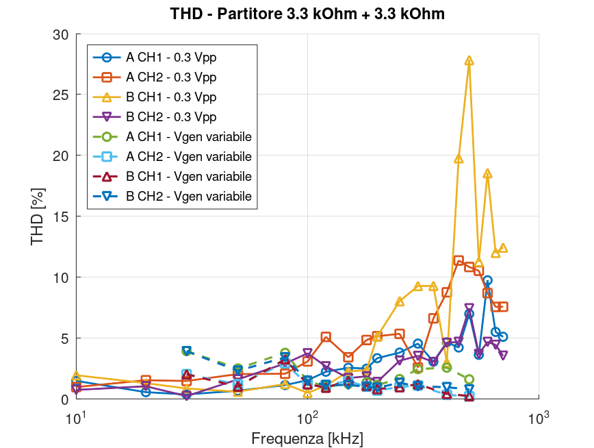
To make the comparison between acquisitions with Fixed Vgen and those with variable Vgen, I also plotted THD as a function of frequency.
The plots separately show the values calculated on the two channels CH1 (VSENSE) and CH2 (VOUT), while also keeping acquisitions A and B. This makes it possible to directly compare, for each divider, the series performed at 300 mVpp with those in which the injection amplitude was adjusted during the measurement.
As can be seen, using an adjustable Vgen generally makes it possible to keep THD lower, especially in the regions where, with 300 mVpp, one of the acquired signals becomes very small.
The following gallery shows the plots for the 3.3 kΩ + 3.3 kΩ and 33 kΩ + 33 kΩ.
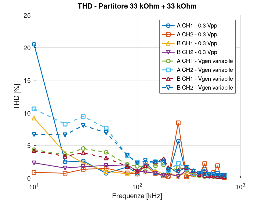 Partitore 33 kΩ + 33 kΩ – THD in funzione della frequenza. Confronto tra le acquisizioni A e B sui canali CH1 (VSENSE) e CH2 (VOUT), per Vgen = 300 mVpp e Vgen variabile. Alle basse frequenze sono particolarmente evidenti gli elevati valori di THD associati alle condizioni in cui uno dei segnali acquisiti presenta ampiezza molto ridotta.
Comparison of the final measurement
In addition to the distortion of the individual signals, it is useful to directly verify how much the choice of Vgen affects the final result obtained after combining measurements A and B.
In the following tables I therefore compare, at the same frequency, the final magnitude and the final phase obtained with Vgen = 300 mVpp and with variable Vgen. To facilitate comparison, the phases are shown on the same branch around +180° when necessary.
3.3 kΩ + 3.3 kΩ divider
The values for the 300 mVpp series and the variable-Vgen series come from the respective tables PROCESSED RESULTS A / B / FINAL.
| Frequency | Final dB 0.3 V | Final phase 0.3 V | Final dB variable Vgen | Final phase variable Vgen |
|---|---|---|---|---|
| 10 kHz | -0.005 | 178.062° | — | — |
| 20 kHz | -0.001 | 180.833° | — | — |
| 30 kHz | -0.017 | 179.912° | -0.340 | 180.035° |
| 50 kHz | -0.039 | 179.646° | -0.274 | 180.337° |
| 80 kHz | -0.180 | 179.411° | -0.294 | 180.366° |
| 100 kHz | -0.165 | 179.401° | -0.251 | 180.415° |
| 120 kHz | -0.093 | 179.118° | -0.236 | 180.435° |
| 150 kHz | +0.108 | 178.849° | -0.219 | 180.564° |
| 180 kHz | +0.041 | 178.630° | -0.216 | 180.633° |
| 200 kHz | +0.090 | 179.672° | -0.230 | 181.034° |
| 250 kHz | +0.123 | 178.867° | -0.184 | 180.635° |
| 300 kHz | +0.090 | 177.930° | -0.145 | 180.620° |
| 350 kHz | +0.445 | 176.261° | — | — |
| 400 kHz | -0.507 | 176.444° | -0.294 | 178.434° |
| 450 kHz | -0.248 | 173.374° | — | — |
| 500 kHz | -0.540 | 174.126° | -0.553 | 179.975° |
| 550 kHz | -0.361 | 176.676° | — | — |
| 600 kHz | -0.473 | 174.744° | — | — |
| 650 kHz | -0.314 | 177.573° | — | — |
| 700 kHz | -0.326 | 177.358° | — | — |
33 kΩ + 33 kΩ divider
Here too, the values Final dB and Final phase from the two campaigns are compared directly.
| Frequency | Final dB 0.3 V | Final phase 0.3 V | Final dB variable Vgen | Final phase variable Vgen |
|---|---|---|---|---|
| 10 kHz | +22.352 | 95.096° | -23.246 | 262.258° |
| 20 kHz | +16.528 | 100.890° | -17.180 | 259.084° |
| 30 kHz | +13.194 | 104.316° | -13.705 | 254.490° |
| 50 kHz | +8.769 | 112.981° | -9.278 | 245.916° |
| 80 kHz | +4.726 | 124.800° | -5.337 | 233.539° |
| 100 kHz | +2.937 | 132.313° | -3.663 | 224.817° |
| 120 kHz | +1.773 | 140.698° | -2.334 | 217.652° |
| 150 kHz | +0.410 | 151.458° | -1.250 | 207.260° |
| 180 kHz | -0.094 | 159.682° | -0.726 | 199.303° |
| 200 kHz | -0.219 | 163.655° | -0.573 | 195.290° |
| 250 kHz | -0.572 | 171.643° | -0.351 | 189.149° |
| 300 kHz | -0.367 | 173.944° | -0.317 | 185.670° |
| 350 kHz | -0.438 | 175.762° | -0.316 | 183.648° |
| 400 kHz | -0.417 | 176.750° | -0.351 | 182.629° |
| 450 kHz | -0.246 | 177.661° | -0.356 | 182.229° |
| 500 kHz | -0.388 | 178.092° | -0.338 | 182.023° |
| 550 kHz | -0.365 | 178.479° | -0.313 | 181.465° |
| 600 kHz | -0.116 | 178.672° | -0.321 | 181.256° |
| 650 kHz | -0.340 | 178.946° | -0.320 | 181.095° |
| 700 kHz | -0.392 | 179.025° | -0.320 | 180.979° |
Direct comparison of the final measurement
To make the comparison between the two test methods more immediate, I used the values reported in the previous tables to build two additional summary plots.
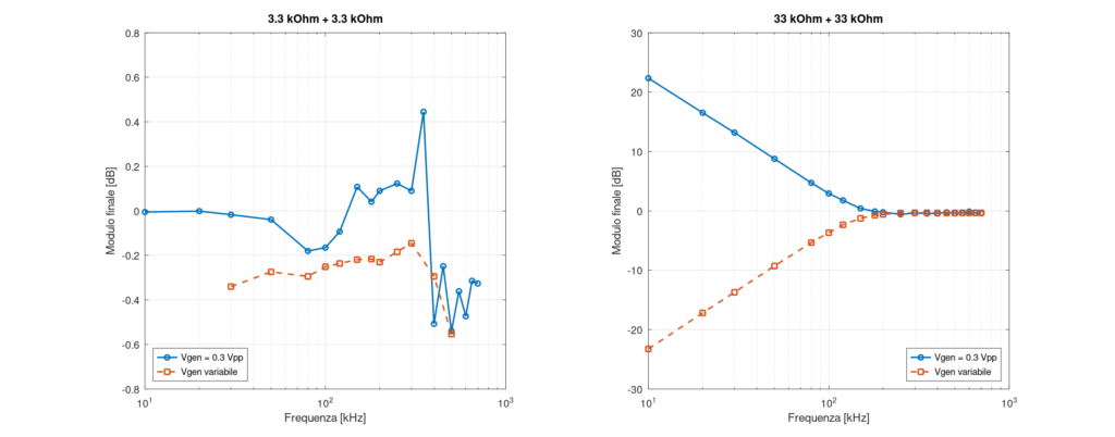
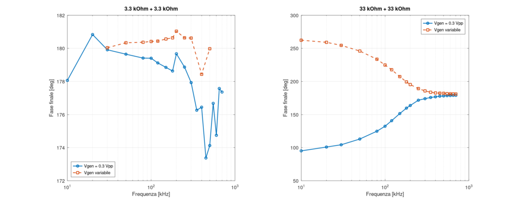
The first shows the final magnitude, the second the final phase. In both cases, the left panel refers to the 3.3 kΩ + 3.3 kΩ divider, while the right panel shows the behavior of the 33 kΩ + 33 kΩ divider. Within each panel, the series performed with Vgen = 300 mVpp is directly compared with the series obtained by adjusting Vgen as a function of frequency.
The plots therefore do not introduce any new data processing: they are simply the frequency-domain representation of the Final dB and Final phase columns reported in the previous tables. For the 3.3 kΩ divider, the variable-Vgen series contains only the frequencies that were actually acquired.
An important detail about the 33 kΩ divider
In the panel for the 33 kΩ + 33 kΩ divider, the two curves appear almost mirror images, especially at low frequencies. This behavior, however, requires clarification.
The orientation of the injection-transformer terminals was not the same in the two measurement campaigns. As a result, in one series the transfer function was evaluated in one orientation, while in the other it was effectively evaluated as its reciprocal.
Denoting by
H = VOUT VSENSEthe transfer function used in the processing, reversing the orientation gives
H′ = 1 HThis does not mean that the magnitude expressed in dB should simply be treated as an absolute value. The linear magnitude |H| is always positive, but its value in decibels is
MdB = 20 log10 |H|and can therefore correctly be either positive or negative.
Taking the reciprocal:
20 log10 1 |H| = -20 log10 |H|so the correct transformation is
M′dB = −MdBSimilarly, the phase changes sign:
φ′=−φ
and can subsequently be shifted by multiples of 360° to place it on the same branch as the other measurement.
The point at 10 kHz is particularly illustrative. In the variable-Vgen campaign, the final result is −23.246 dB and −97.742°. Correcting the orientation gives:
+23.246 dB, +97.742°
while the measurement performed at 300 mVpp gives +22.352 dB and +95.096°. The two results are therefore very close, even though they appear on opposite sides in the raw plot. The original values of the two series are those returned directly by the A/B processing.
The same phenomenon continues at higher frequencies. As the frequency increases, both campaigns converge toward 0 dB and 180°, and the difference caused by orientation becomes progressively less visible.
I nevertheless kept the values in the plots exactly as obtained in the two campaigns rather than retroactively correcting one of the curves. In this way the figure faithfully documents the acquired data; in the interpretation, however, a correct comparison for the 33 kΩ divider requires accounting for the reversed orientation.
What the two plots show
For the 3.3 kΩ + 3.3 kΩ divider, where the orientation can be compared directly, the two campaigns provide relatively close final values despite the large difference in the Vgen amplitude used. In particular, the variable-Vgen series remains very close to 0 dB and 180° even when the injection signal is increased substantially.
For the 33 kΩ + 33 kΩ divider, however, directly reading the two curves is misleading until the inversion of the ratio is taken into account. Once the H→1/H transformation is mentally applied, a much closer correspondence between the two campaigns emerges here as well.
These plots are therefore useful for two distinct reasons: they show at a glance the effect of changing Vgen on the final result and, at the same time, highlight how important it is to maintain—or at least record—the transformer orientation and the transfer-function convention when comparing acquisitions made in different sessions.
Standardizing the A/B orientation
These tests also highlighted the need to make the injection-transformer orientation unambiguous. To prevent the reversal observed in the previous data from recurring in future campaigns, I therefore permanently labeled the two secondary terminals A and B and established a fixed convention for all subsequent acquisitions.
I will always consider OUT as the high side of the network and SENS as the low side. The convention will therefore be:
- measurement A: transformer terminal A connected to OUT and terminal B connected to SENS;
- measurement B: terminal B connected to OUT and terminal A connected to SENS.
In this way, future A and B series will always have the same meaning, and plots obtained in different sessions can be compared directly without having to reconstruct the orientation used afterward.
A first conclusion about injection amplitude
The main result of this work session concerns the choice of injection-signal amplitude.
Initially I had decided to use Vgen = 300 mVpp in all measurements, thinking that keeping the generator amplitude constant would help make the different tests comparable. Today’s results instead indicate that this precaution is unnecessary and, under some conditions, can even be counterproductive.
When Vgen is too low, one of the two acquired signals can fall to a few tens of millivolts or even less. Under these conditions the relative contribution of noise increases and the harmonic analysis becomes less clean. The THD plots show that, in general, acquisitions performed using a Vgen adjusted as a function of frequency show lower distortion values than the corresponding measurements performed with the generator kept at 300 mVpp.
At the same time, comparison of the final results shows that increasing Vgen, as long as the system remains in its linear region, does not significantly alter the transfer function I am trying to measure. I can therefore use a higher injection signal to obtain larger-amplitude waveforms and a better signal-to-noise ratio, without being forced to work with signals of only about 20 mV.
The procedure I will adopt from now on will therefore be to progressively increase Vgen before acquisition, looking for the highest usable level without entering a nonlinear condition. Harmonic analysis also provides a quantitative check: if increasing the amplitude begins to produce real distortion, it becomes visible through the increase in harmonic components and THD.
The practical conclusion from this first part of the characterization is therefore that Vgen does not necessarily have to be kept constant. It is preferable to adapt it to the measurement conditions, using a level high enough to obtain clean, easily measurable signals while remaining below the threshold at which distortion begins to appear.
The second issue that emerged during the tests remains open: the dependence of the measurement on DUT impedance. This will be the subject of the next characterization phase, again using the calibration bench to better understand the origin of the error and how to manage it.