

GX LII-2 – Lab Log: Bode Measurement Campaign on Resistive Dividers
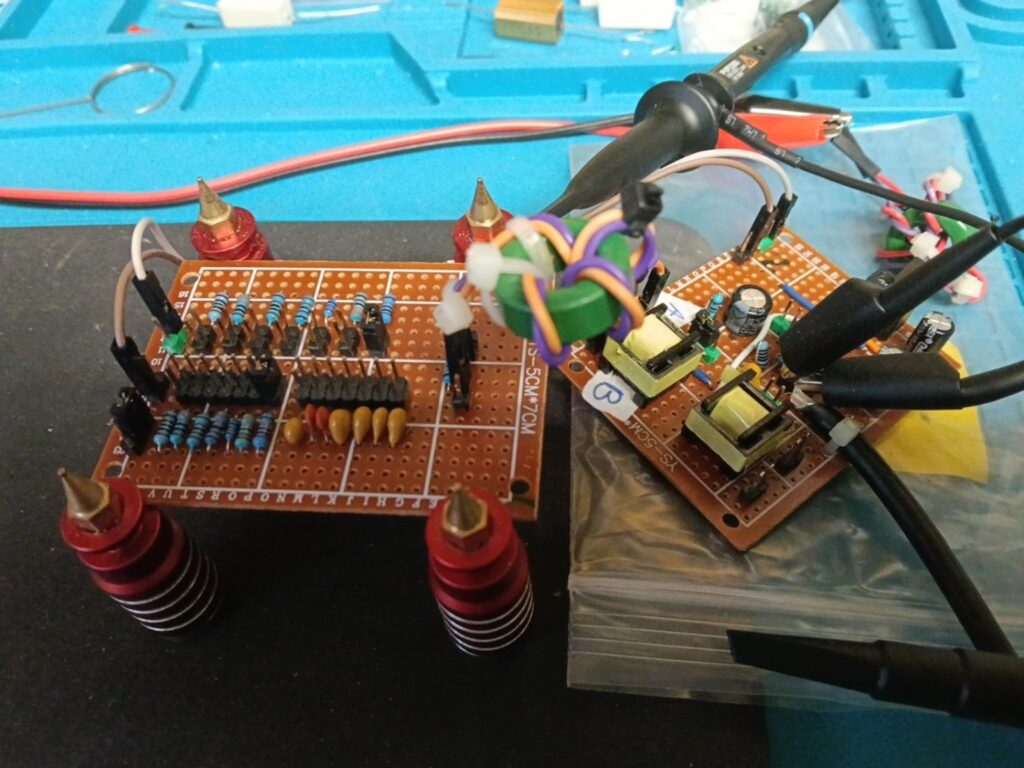
Before discussing the results of this new measurement campaign, I am linking the first article in the series here, where I described the starting point of the GX LII-2 project, the experimental test bench, and the first characterization tests. Since then, the measurement method, the setup, and especially the data processing have changed considerably.
A measurement campaign more demanding than expected
This campaign proved quite demanding, mainly because the signals measured at the OUT and SENSE nodes are very small. Even under the most favorable conditions, peak-to-peak amplitudes are often only a few tens of millivolts, so careful setup becomes essential.
When a measurement is only intended to give a general idea of a circuit’s behavior, some compromises can be accepted; in this case, however, I am collecting data that I want to use to characterize the system properly. The final error results from the sum of many small contributions, so it becomes necessary to eliminate them, or at least reduce them, one at a time.
For this reason, during the acquisitions I chose to switch off practically all unnecessary electronics in the laboratory, including the LED lighting, and worked with a battery-powered lamp. I also paid close attention to the routing of power and signal cables and used high-permeability ferrite rings on the connections, with the aim of increasing the impedance to common-mode currents and further reducing interference introduced into the measurement system.
Despite these precautions, a residual low-frequency component remains visible, roughly in the 50–100 Hz range. Its origin still needs to be verified: it could be common-mode interference or a signal actually injected by some element of the setup.
Fortunately, the processing I use in GNU Octave does not derive magnitude and phase directly from the overall waveform amplitude, but instead extracts the component at the injection frequency by fitting. A 50 or 100 Hz disturbance is therefore not directly confused with the fundamental I am measuring, and its contribution to the final result is greatly reduced.
This does not make careful setup unnecessary; on the contrary, I still prefer to start with signals that are as clean as possible. Fitting is an additional safeguard against unwanted components, not a reason to neglect measurement quality.
Scope of this campaign
Seven resistive pairs, from 100 Ω to 100 kΩ, were characterized at 30 frequencies between 10 kHz and 700 kHz, performing both A and B acquisitions at every point. The injection branch uses Rinj = 18 Ω; CH1 measures VSENSE and CH2 measures VOUT. Vgen was not kept constant throughout the sweep, but adjusted point by point to maintain an adequate signal level while remaining in the linear region.
The LTspice trace used for comparison represents the ideal circuit built with the actual measured resistance values. I did not include capacitances, inductances, or other parasitic elements of the fixture and transformer in the model; the frequency-dependent structures that emerge experimentally are therefore not already incorporated into the simulated reference.
Measurement campaign data
Before moving on to the Bode plots, I report the data used for this campaign. The first table is the same one already presented in the first article of the series and contains the actual measured resistor values on the calibration bench. I include it again here for convenience because these values, rather than the nominal ones, are used as the reference in the subsequent processing and simulations.
| Nominal series | Upper R [Ω] | Lower R [Ω] | Rupper/Rlower |
|---|---|---|---|
| 100R | 99.94 | 99.70 | 1.002407 |
| 330R | 323.80 | 324.40 | 0.998150 |
| 1k | 995.70 | 999.00 | 0.996697 |
| 3.3k | 3260.00 | 3290.00 | 0.990881 |
| 10k | 9800.00 | 10010.00 | 0.979021 |
| 33k | 32990.00 | 32940.00 | 1.001518 |
| 100k | 99770.00 | 99330.00 | 1.004430 |
For each resistive combination, I then collected in a second table the fundamental levels actually measured at the SENSE and OUT nodes, keeping the A and B acquisitions separate.
For each point, the table contains the nominal series value, the actual values of upper R and lower R, the measurement frequency, and the fundamental amplitudes obtained from the GNU Octave fit, expressed both as Vpk and Vpp.
The columns are therefore:
serie_nominale — divider identificationR_alto_ohm — actual upper-resistor valueR_basso_ohm — actual lower-resistor valuef_Hz — measurement frequencyVSENSE_A_Vpk, VSENSE_A_Vpp — fundamental at SENSE, measurement AVOUT_A_Vpk, VOUT_A_Vpp — fundamental at OUT, measurement AVSENSE_B_Vpk, VSENSE_B_Vpp — fundamental at SENSE, measurement BVOUT_B_Vpk, VOUT_B_Vpp — fundamental at OUT, measurement B
Complete VSENSE and VOUT amplitude table
| serie_nominale | R_alto_ohm | R_basso_ohm | f_Hz | VSENSE_A_Vpk | VSENSE_A_Vpp | VOUT_A_Vpk | VOUT_A_Vpp | VSENSE_B_Vpk | VSENSE_B_Vpp | VOUT_B_Vpk | VOUT_B_Vpp |
|---|---|---|---|---|---|---|---|---|---|---|---|
| 100R | 99.94 | 99.7 | 10000 | 0.051966553 | 0.103933106 | 0.0515555058 | 0.103111012 | 0.0513025477 | 0.102605095 | 0.0522774051 | 0.10455481 |
| 100R | 99.94 | 99.7 | 20000 | 0.0506356116 | 0.101271223 | 0.050048633 | 0.100097266 | 0.0499897897 | 0.0999795794 | 0.0507702399 | 0.10154048 |
| 100R | 99.94 | 99.7 | 30000 | 0.0494554846 | 0.0989109692 | 0.0473021597 | 0.0946043194 | 0.0475143672 | 0.0950287344 | 0.0493570395 | 0.098714079 |
| 100R | 99.94 | 99.7 | 50000 | 0.0509689175 | 0.101937835 | 0.0476714068 | 0.0953428137 | 0.0479383926 | 0.0958767851 | 0.0511129995 | 0.102225999 |
| 100R | 99.94 | 99.7 | 80000 | 0.0527978907 | 0.105595781 | 0.0477935012 | 0.0955870024 | 0.0482230661 | 0.0964461323 | 0.0530146409 | 0.106029282 |
| 100R | 99.94 | 99.7 | 100000 | 0.0559861529 | 0.111972306 | 0.0499663426 | 0.0999326852 | 0.0504354713 | 0.100870943 | 0.0562623129 | 0.112524626 |
| 100R | 99.94 | 99.7 | 120000 | 0.049914423 | 0.099828846 | 0.0440890364 | 0.0881780729 | 0.0445418221 | 0.0890836442 | 0.0502048651 | 0.10040973 |
| 100R | 99.94 | 99.7 | 140000 | 0.0588979736 | 0.117795947 | 0.0515834148 | 0.10316683 | 0.0521876548 | 0.10437531 | 0.0592600831 | 0.118520166 |
| 100R | 99.94 | 99.7 | 160000 | 0.0502158428 | 0.100431686 | 0.0436936644 | 0.0873873288 | 0.044231718 | 0.0884634359 | 0.0504719501 | 0.1009439 |
| 100R | 99.94 | 99.7 | 180000 | 0.0395268263 | 0.0790536526 | 0.0342196614 | 0.0684393229 | 0.0346156675 | 0.0692313351 | 0.0397271449 | 0.0794542898 |
| 100R | 99.94 | 99.7 | 200000 | 0.0276955015 | 0.0553910031 | 0.0238474054 | 0.0476948108 | 0.0241639349 | 0.0483278698 | 0.0278573273 | 0.0557146546 |
| 100R | 99.94 | 99.7 | 220000 | 0.025492782 | 0.0509855639 | 0.0218417041 | 0.0436834081 | 0.022136888 | 0.044273776 | 0.0256280189 | 0.0512560379 |
| 100R | 99.94 | 99.7 | 240000 | 0.023608973 | 0.047217946 | 0.0201373159 | 0.0402746317 | 0.0204045315 | 0.040809063 | 0.0237110497 | 0.0474220993 |
| 100R | 99.94 | 99.7 | 260000 | 0.0219702783 | 0.0439405566 | 0.018660442 | 0.037320884 | 0.0189113024 | 0.0378226047 | 0.0220626597 | 0.0441253194 |
| 100R | 99.94 | 99.7 | 280000 | 0.0205535065 | 0.0411070129 | 0.0173633265 | 0.0347266531 | 0.017604651 | 0.035209302 | 0.0206294032 | 0.0412588063 |
| 100R | 99.94 | 99.7 | 300000 | 0.0233136481 | 0.0466272962 | 0.0196198484 | 0.0392396968 | 0.0198870685 | 0.0397741369 | 0.0234079529 | 0.0468159059 |
| 100R | 99.94 | 99.7 | 320000 | 0.0219787825 | 0.0439575649 | 0.0184149116 | 0.0368298232 | 0.0186666627 | 0.0373333253 | 0.0220673428 | 0.0441346855 |
| 100R | 99.94 | 99.7 | 350000 | 0.0202453704 | 0.0404907407 | 0.0168379481 | 0.0336758962 | 0.0170927733 | 0.0341855466 | 0.0203137952 | 0.0406275905 |
| 100R | 99.94 | 99.7 | 370000 | 0.0192402603 | 0.0384805206 | 0.0159190311 | 0.0318380622 | 0.0161690839 | 0.0323381679 | 0.0193039335 | 0.0386078669 |
| 100R | 99.94 | 99.7 | 400000 | 0.01792498 | 0.03584996 | 0.0146925231 | 0.0293850462 | 0.0149334379 | 0.0298668758 | 0.0179723354 | 0.0359446707 |
| 100R | 99.94 | 99.7 | 430000 | 0.0280098345 | 0.056019669 | 0.0227780537 | 0.0455561073 | 0.0231522252 | 0.0463044504 | 0.0281223406 | 0.0562446811 |
| 100R | 99.94 | 99.7 | 450000 | 0.0268774008 | 0.0537548015 | 0.0217092236 | 0.0434184473 | 0.0220928692 | 0.0441857384 | 0.0269780335 | 0.053956067 |
| 100R | 99.94 | 99.7 | 480000 | 0.0253584764 | 0.0507169527 | 0.0202896989 | 0.0405793978 | 0.0206599336 | 0.0413198673 | 0.025430841 | 0.050861682 |
| 100R | 99.94 | 99.7 | 500000 | 0.0244414339 | 0.0488828678 | 0.0194292123 | 0.0388584247 | 0.0197967133 | 0.0395934267 | 0.0244920466 | 0.0489840932 |
| 100R | 99.94 | 99.7 | 530000 | 0.0232105687 | 0.0464211374 | 0.0182452706 | 0.0364905411 | 0.0186006739 | 0.0372013478 | 0.0232410388 | 0.0464820775 |
| 100R | 99.94 | 99.7 | 550000 | 0.0224518289 | 0.0449036579 | 0.0175321079 | 0.0350642159 | 0.0178801783 | 0.0357603565 | 0.0224793745 | 0.044958749 |
| 100R | 99.94 | 99.7 | 580000 | 0.0214174038 | 0.0428348077 | 0.0165395117 | 0.0330790233 | 0.0168780749 | 0.0337561498 | 0.0214406191 | 0.0428812382 |
| 100R | 99.94 | 99.7 | 600000 | 0.0207898229 | 0.0415796458 | 0.0159268442 | 0.0318536884 | 0.0162486214 | 0.0324972427 | 0.0208195107 | 0.0416390215 |
| 100R | 99.94 | 99.7 | 650000 | 0.0194041859 | 0.0388083718 | 0.0145557463 | 0.0291114927 | 0.0148469906 | 0.0296939812 | 0.0194335371 | 0.0388670743 |
| 100R | 99.94 | 99.7 | 700000 | 0.0182233133 | 0.0364466266 | 0.0133790917 | 0.0267581835 | 0.0136210037 | 0.0272420075 | 0.018252781 | 0.0365055619 |
| 330R | 323.8 | 324.4 | 10000 | 0.0418762407 | 0.0837524813 | 0.0404807357 | 0.0809614715 | 0.0408110775 | 0.081622155 | 0.0415780428 | 0.0831560857 |
| 330R | 323.8 | 324.4 | 20000 | 0.0405245034 | 0.0810490068 | 0.0395173709 | 0.0790347418 | 0.039659541 | 0.079319082 | 0.0404256591 | 0.0808513182 |
| 330R | 323.8 | 324.4 | 30000 | 0.0395216434 | 0.0790432867 | 0.0372714988 | 0.0745429975 | 0.0374805726 | 0.0749611453 | 0.0392953406 | 0.0785906813 |
| 330R | 323.8 | 324.4 | 50000 | 0.0475689374 | 0.0951378748 | 0.0434203772 | 0.0868407544 | 0.0436747197 | 0.0873494394 | 0.0474453475 | 0.094890695 |
| 330R | 323.8 | 324.4 | 80000 | 0.0398270268 | 0.0796540536 | 0.0348495694 | 0.0696991389 | 0.0350817298 | 0.0701634596 | 0.0397021032 | 0.0794042063 |
| 330R | 323.8 | 324.4 | 100000 | 0.0404123623 | 0.0808247246 | 0.0346212808 | 0.0692425616 | 0.0348511627 | 0.0697023254 | 0.0401954808 | 0.0803909616 |
| 330R | 323.8 | 324.4 | 120000 | 0.0358552807 | 0.0717105614 | 0.0302927262 | 0.0605854523 | 0.0304927767 | 0.0609855535 | 0.0357407323 | 0.0714814647 |
| 330R | 323.8 | 324.4 | 140000 | 0.0442760754 | 0.0885521509 | 0.0369614574 | 0.0739229148 | 0.037215346 | 0.0744306921 | 0.044110411 | 0.088220822 |
| 330R | 323.8 | 324.4 | 160000 | 0.0399609389 | 0.0799218779 | 0.0330130076 | 0.0660260152 | 0.0332486297 | 0.0664972593 | 0.0398015503 | 0.0796031005 |
| 330R | 323.8 | 324.4 | 180000 | 0.039738001 | 0.0794760021 | 0.0324884117 | 0.0649768235 | 0.0327498377 | 0.0654996754 | 0.0395442671 | 0.0790885343 |
| 330R | 323.8 | 324.4 | 200000 | 0.0455223719 | 0.0910447438 | 0.0368274845 | 0.0736549691 | 0.0371411353 | 0.0742822706 | 0.0453226029 | 0.0906452058 |
| 330R | 323.8 | 324.4 | 220000 | 0.0420486429 | 0.0840972857 | 0.0336606512 | 0.0673213023 | 0.0339643951 | 0.0679287903 | 0.0418159318 | 0.0836318635 |
| 330R | 323.8 | 324.4 | 240000 | 0.0390313647 | 0.0780627295 | 0.0309337406 | 0.0618674812 | 0.0312481949 | 0.0624963898 | 0.0388237176 | 0.0776474352 |
| 330R | 323.8 | 324.4 | 260000 | 0.0364372712 | 0.0728745423 | 0.0285492486 | 0.0570984972 | 0.0288856282 | 0.0577712565 | 0.0362600122 | 0.0725200244 |
| 330R | 323.8 | 324.4 | 280000 | 0.0364523745 | 0.0729047491 | 0.0282381678 | 0.0564763357 | 0.0285783444 | 0.0571566889 | 0.0362505312 | 0.0725010623 |
| 330R | 323.8 | 324.4 | 300000 | 0.0343707586 | 0.0687415171 | 0.0262738582 | 0.0525477163 | 0.0266403766 | 0.0532807531 | 0.0341594658 | 0.0683189316 |
| 330R | 323.8 | 324.4 | 320000 | 0.0324912 | 0.0649824 | 0.0245549932 | 0.0491099863 | 0.0249120675 | 0.0498241351 | 0.0322754202 | 0.0645508405 |
| 330R | 323.8 | 324.4 | 350000 | 0.0301105038 | 0.0602210076 | 0.0222940425 | 0.044588085 | 0.022641276 | 0.0452825521 | 0.029902042 | 0.0598040841 |
| 330R | 323.8 | 324.4 | 370000 | 0.0287389113 | 0.0574778227 | 0.0209506433 | 0.0419012865 | 0.0212877587 | 0.0425755174 | 0.0285065202 | 0.0570130403 |
| 330R | 323.8 | 324.4 | 400000 | 0.0336664974 | 0.0673329949 | 0.0240116039 | 0.0480232079 | 0.0244197594 | 0.0488395187 | 0.0334270942 | 0.0668541884 |
| 330R | 323.8 | 324.4 | 430000 | 0.0317552866 | 0.0635105732 | 0.0220756141 | 0.0441512283 | 0.0224506134 | 0.0449012268 | 0.0314826379 | 0.0629652757 |
| 330R | 323.8 | 324.4 | 450000 | 0.0306048337 | 0.0612096674 | 0.0209135917 | 0.0418271833 | 0.0212663088 | 0.0425326175 | 0.0303482018 | 0.0606964035 |
| 330R | 323.8 | 324.4 | 480000 | 0.0290642991 | 0.0581285982 | 0.0193310001 | 0.0386620002 | 0.0196650451 | 0.0393300901 | 0.0288157051 | 0.0576314102 |
| 330R | 323.8 | 324.4 | 500000 | 0.028138283 | 0.0562765659 | 0.0183697697 | 0.0367395395 | 0.0186787432 | 0.0373574864 | 0.0279013521 | 0.0558027042 |
| 330R | 323.8 | 324.4 | 530000 | 0.0269123324 | 0.0538246647 | 0.0170420641 | 0.0340841281 | 0.0173353043 | 0.0346706085 | 0.0266674874 | 0.0533349749 |
| 330R | 323.8 | 324.4 | 550000 | 0.0261751262 | 0.0523502523 | 0.016230725 | 0.03246145 | 0.0165145654 | 0.0330291307 | 0.0259257495 | 0.051851499 |
| 330R | 323.8 | 324.4 | 580000 | 0.0251710155 | 0.0503420309 | 0.0150924964 | 0.0301849929 | 0.0153589463 | 0.0307178925 | 0.0249364459 | 0.0498728919 |
| 330R | 323.8 | 324.4 | 600000 | 0.0245621209 | 0.0491242418 | 0.0143932561 | 0.0287865122 | 0.0146442177 | 0.0292884354 | 0.0243388419 | 0.0486776838 |
| 330R | 323.8 | 324.4 | 650000 | 0.0232315329 | 0.0464630658 | 0.0128056079 | 0.0256112158 | 0.0130185019 | 0.0260370038 | 0.0230153581 | 0.0460307162 |
| 330R | 323.8 | 324.4 | 700000 | 0.0221244983 | 0.0442489966 | 0.0114019007 | 0.0228038014 | 0.0115880516 | 0.0231761032 | 0.0219197229 | 0.0438394457 |
| 1k | 995.7 | 999.0 | 10000 | 0.0419000115 | 0.0838000229 | 0.0413704171 | 0.0827408342 | 0.0408546883 | 0.0817093766 | 0.0423031459 | 0.0846062919 |
| 1k | 995.7 | 999.0 | 20000 | 0.0416064301 | 0.0832128602 | 0.0393727837 | 0.0787455675 | 0.0392598552 | 0.0785197105 | 0.0416411308 | 0.0832822617 |
| 1k | 995.7 | 999.0 | 30000 | 0.0401725698 | 0.0803451395 | 0.0375577629 | 0.0751155259 | 0.0372363507 | 0.0744727013 | 0.0403844152 | 0.0807688304 |
| 1k | 995.7 | 999.0 | 50000 | 0.0491366155 | 0.098273231 | 0.0430924737 | 0.0861849473 | 0.043214237 | 0.086428474 | 0.0489707617 | 0.0979415234 |
| 1k | 995.7 | 999.0 | 80000 | 0.0415190935 | 0.083038187 | 0.0342922514 | 0.0685845029 | 0.0345399632 | 0.0690799263 | 0.0412273992 | 0.0824547983 |
| 1k | 995.7 | 999.0 | 100000 | 0.0474441692 | 0.0948883385 | 0.0381229801 | 0.0762459603 | 0.0385433833 | 0.0770867667 | 0.0470544747 | 0.0941089493 |
| 1k | 995.7 | 999.0 | 120000 | 0.0423698339 | 0.0847396677 | 0.0331849344 | 0.0663698688 | 0.0336665609 | 0.0673331219 | 0.0419267216 | 0.0838534432 |
| 1k | 995.7 | 999.0 | 140000 | 0.0467435674 | 0.0934871347 | 0.0358198767 | 0.0716397534 | 0.0363953637 | 0.0727907273 | 0.0462171741 | 0.0924343482 |
| 1k | 995.7 | 999.0 | 160000 | 0.04240372 | 0.08480744 | 0.0317644534 | 0.0635289068 | 0.0323394671 | 0.0646789341 | 0.0418832226 | 0.0837664453 |
| 1k | 995.7 | 999.0 | 180000 | 0.038807157 | 0.077614314 | 0.0283878891 | 0.0567757781 | 0.0289638678 | 0.0579277356 | 0.0383043644 | 0.0766087289 |
| 1k | 995.7 | 999.0 | 200000 | 0.0456516132 | 0.0913032264 | 0.0325602689 | 0.0651205379 | 0.0332614726 | 0.0665229452 | 0.045029759 | 0.0900595179 |
| 1k | 995.7 | 999.0 | 220000 | 0.0424032775 | 0.084806555 | 0.0294639015 | 0.0589278029 | 0.0301599497 | 0.0603198994 | 0.0418054754 | 0.0836109508 |
| 1k | 995.7 | 999.0 | 240000 | 0.0396566377 | 0.0793132753 | 0.0267950583 | 0.0535901166 | 0.0274418236 | 0.0548836472 | 0.0390777643 | 0.0781555286 |
| 1k | 995.7 | 999.0 | 260000 | 0.0372779516 | 0.0745559032 | 0.0244527186 | 0.0489054372 | 0.0250721884 | 0.0501443768 | 0.0367706016 | 0.0735412031 |
| 1k | 995.7 | 999.0 | 280000 | 0.0377396316 | 0.0754792632 | 0.0239612467 | 0.0479224934 | 0.0245861714 | 0.0491723428 | 0.0372355043 | 0.0744710086 |
| 1k | 995.7 | 999.0 | 300000 | 0.0358602622 | 0.0717205244 | 0.0219823937 | 0.0439647875 | 0.0225772303 | 0.0451544605 | 0.0353793867 | 0.0707587735 |
| 1k | 995.7 | 999.0 | 320000 | 0.034235814 | 0.068471628 | 0.0201993642 | 0.0403987285 | 0.020779757 | 0.0415595139 | 0.0337401253 | 0.0674802505 |
| 1k | 995.7 | 999.0 | 350000 | 0.0321670629 | 0.0643341259 | 0.0178649791 | 0.0357299582 | 0.0183900392 | 0.0367800784 | 0.031653779 | 0.0633075581 |
| 1k | 995.7 | 999.0 | 370000 | 0.0413367899 | 0.0826735797 | 0.0219912357 | 0.0439824714 | 0.0226465411 | 0.0452930822 | 0.0407033803 | 0.0814067605 |
| 1k | 995.7 | 999.0 | 400000 | 0.0392987816 | 0.0785975632 | 0.019447393 | 0.0388947861 | 0.0200808363 | 0.0401616725 | 0.0386832369 | 0.0773664739 |
| 1k | 995.7 | 999.0 | 430000 | 0.0375980728 | 0.0751961455 | 0.0172173556 | 0.0344347113 | 0.0178311 | 0.0356622 | 0.0370153317 | 0.0740306635 |
| 1k | 995.7 | 999.0 | 450000 | 0.0366140624 | 0.0732281248 | 0.0158617042 | 0.0317234085 | 0.0164388516 | 0.0328777032 | 0.036069803 | 0.072139606 |
| 1k | 995.7 | 999.0 | 480000 | 0.0407425952 | 0.0814851903 | 0.0161313872 | 0.0322627743 | 0.0167427689 | 0.0334855378 | 0.0400698776 | 0.0801397552 |
| 1k | 995.7 | 999.0 | 500000 | 0.0398542091 | 0.0797084183 | 0.0148147139 | 0.0296294279 | 0.0153884871 | 0.0307769743 | 0.0392340896 | 0.0784681792 |
| 1k | 995.7 | 999.0 | 530000 | 0.0387438874 | 0.0774877749 | 0.0129558456 | 0.0259116912 | 0.0135289169 | 0.0270578337 | 0.0381438688 | 0.0762877377 |
| 1k | 995.7 | 999.0 | 550000 | 0.0381216891 | 0.0762433783 | 0.011825677 | 0.023651354 | 0.0123964357 | 0.0247928714 | 0.0375138396 | 0.0750276792 |
| 1k | 995.7 | 999.0 | 580000 | 0.0372568412 | 0.0745136824 | 0.010258084 | 0.0205161681 | 0.0107887561 | 0.0215775122 | 0.0366679401 | 0.0733358803 |
| 1k | 995.7 | 999.0 | 600000 | 0.0367686803 | 0.0735373605 | 0.0092869489 | 0.0185738978 | 0.00980695812 | 0.0196139162 | 0.0361959572 | 0.0723919143 |
| 1k | 995.7 | 999.0 | 650000 | 0.0357663497 | 0.0715326994 | 0.00713220303 | 0.0142644061 | 0.0076536363 | 0.0153072726 | 0.0351905321 | 0.0703810642 |
| 1k | 995.7 | 999.0 | 700000 | 0.0350019455 | 0.0700038911 | 0.00542605664 | 0.0108521133 | 0.00588701601 | 0.011774032 | 0.0344289803 | 0.0688579606 |
| 3.3k | 3260.0 | 3290.0 | 10000 | 0.0563444615 | 0.112688923 | 0.0537835744 | 0.107567149 | 0.0543001961 | 0.108600392 | 0.0558448659 | 0.111689732 |
| 3.3k | 3260.0 | 3290.0 | 20000 | 0.0553259529 | 0.110651906 | 0.051950211 | 0.103900422 | 0.052342732 | 0.104685464 | 0.0549387142 | 0.109877428 |
| 3.3k | 3260.0 | 3290.0 | 30000 | 0.0546120631 | 0.109224126 | 0.0485446575 | 0.0970893151 | 0.0490009918 | 0.0980019835 | 0.0541709037 | 0.108341807 |
| 3.3k | 3260.0 | 3290.0 | 50000 | 0.0506495962 | 0.101299192 | 0.0418947731 | 0.0837895462 | 0.0424452799 | 0.0848905598 | 0.0502242746 | 0.100448549 |
| 3.3k | 3260.0 | 3290.0 | 80000 | 0.049397655 | 0.09879531 | 0.037826069 | 0.075652138 | 0.038363353 | 0.076726706 | 0.0488447465 | 0.0976894929 |
| 3.3k | 3260.0 | 3290.0 | 100000 | 0.0442456109 | 0.0884912217 | 0.032304996 | 0.0646099919 | 0.0328580245 | 0.065716049 | 0.0437281725 | 0.087456345 |
| 3.3k | 3260.0 | 3290.0 | 120000 | 0.0447804549 | 0.0895609097 | 0.0311911163 | 0.0623822327 | 0.0318184152 | 0.0636368304 | 0.0442445148 | 0.0884890296 |
| 3.3k | 3260.0 | 3290.0 | 140000 | 0.0452691797 | 0.0905383594 | 0.0299142201 | 0.0598284402 | 0.0305576078 | 0.0611152155 | 0.0447114366 | 0.0894228732 |
| 3.3k | 3260.0 | 3290.0 | 160000 | 0.0416497187 | 0.0832994374 | 0.0259431074 | 0.0518862148 | 0.026568872 | 0.053137744 | 0.04103857 | 0.0820771401 |
| 3.3k | 3260.0 | 3290.0 | 180000 | 0.0467149883 | 0.0934299767 | 0.027260538 | 0.054521076 | 0.0279683533 | 0.0559367067 | 0.046025326 | 0.092050652 |
| 3.3k | 3260.0 | 3290.0 | 200000 | 0.0437987564 | 0.0875975128 | 0.0237631831 | 0.0475263662 | 0.0244717425 | 0.0489434851 | 0.0431243122 | 0.0862486244 |
| 3.3k | 3260.0 | 3290.0 | 220000 | 0.0483232332 | 0.0966464665 | 0.0242452055 | 0.048490411 | 0.0250041611 | 0.0500083222 | 0.0475335675 | 0.095067135 |
| 3.3k | 3260.0 | 3290.0 | 240000 | 0.0460295487 | 0.0920590973 | 0.0211443934 | 0.0422887868 | 0.0218972315 | 0.0437944629 | 0.0452585989 | 0.0905171977 |
| 3.3k | 3260.0 | 3290.0 | 260000 | 0.0440969334 | 0.0881938667 | 0.0184582629 | 0.0369165259 | 0.0191519076 | 0.0383038153 | 0.0433352491 | 0.0866704982 |
| 3.3k | 3260.0 | 3290.0 | 280000 | 0.0455507894 | 0.0911015789 | 0.0171633034 | 0.0343266067 | 0.0179230453 | 0.0358460905 | 0.0447110349 | 0.0894220699 |
| 3.3k | 3260.0 | 3290.0 | 300000 | 0.0441520403 | 0.0883040806 | 0.0148944586 | 0.0297889172 | 0.0156380002 | 0.0312760004 | 0.0432995302 | 0.0865990603 |
| 3.3k | 3260.0 | 3290.0 | 320000 | 0.0429796286 | 0.0859592572 | 0.0129161212 | 0.0258322424 | 0.0136094846 | 0.0272189691 | 0.042094382 | 0.084188764 |
| 3.3k | 3260.0 | 3290.0 | 350000 | 0.0470963533 | 0.0941927066 | 0.011845466 | 0.023690932 | 0.0125740921 | 0.0251481842 | 0.0461154 | 0.0922308 |
| 3.3k | 3260.0 | 3290.0 | 370000 | 0.0462521102 | 0.0925042204 | 0.0103880207 | 0.0207760415 | 0.0110682935 | 0.022136587 | 0.045270072 | 0.0905401439 |
| 3.3k | 3260.0 | 3290.0 | 400000 | 0.0533450066 | 0.106690013 | 0.0104269217 | 0.0208538435 | 0.0111044291 | 0.0222088583 | 0.0521234278 | 0.104246856 |
| 3.3k | 3260.0 | 3290.0 | 430000 | 0.0524672588 | 0.104934518 | 0.00974848624 | 0.0194969725 | 0.010216842 | 0.020433684 | 0.0512434046 | 0.102486809 |
| 3.3k | 3260.0 | 3290.0 | 450000 | 0.0520325644 | 0.104065129 | 0.00986670852 | 0.019733417 | 0.0101668109 | 0.0203336218 | 0.050796664 | 0.101593328 |
| 3.3k | 3260.0 | 3290.0 | 480000 | 0.064529127 | 0.129058254 | 0.013416825 | 0.0268336499 | 0.0134916187 | 0.0269832374 | 0.0629625605 | 0.125925121 |
| 3.3k | 3260.0 | 3290.0 | 500000 | 0.0642402939 | 0.128480588 | 0.0144877011 | 0.0289754022 | 0.0144439191 | 0.0288878383 | 0.062681439 | 0.125362878 |
| 3.3k | 3260.0 | 3290.0 | 530000 | 0.0639976762 | 0.127995352 | 0.0164557661 | 0.0329115321 | 0.0162589521 | 0.0325179042 | 0.0623851178 | 0.124770236 |
| 3.3k | 3260.0 | 3290.0 | 550000 | 0.063933789 | 0.127867578 | 0.0178949807 | 0.0357899615 | 0.0176019053 | 0.0352038106 | 0.0622720339 | 0.124544068 |
| 3.3k | 3260.0 | 3290.0 | 580000 | 0.0638969125 | 0.127793825 | 0.0201211815 | 0.040242363 | 0.0197376821 | 0.0394753643 | 0.0622146385 | 0.124429277 |
| 3.3k | 3260.0 | 3290.0 | 600000 | 0.0639170617 | 0.127834123 | 0.0216071419 | 0.0432142839 | 0.021149547 | 0.042299094 | 0.0621992403 | 0.124398481 |
| 3.3k | 3260.0 | 3290.0 | 650000 | 0.0642350564 | 0.128470113 | 0.0253322098 | 0.0506644196 | 0.0247670391 | 0.0495340782 | 0.0624211406 | 0.124842281 |
| 3.3k | 3260.0 | 3290.0 | 700000 | 0.0647082209 | 0.129416442 | 0.0288847415 | 0.0577694829 | 0.0282953239 | 0.0565906479 | 0.0628688508 | 0.125737702 |
| 10k | 9800.0 | 10010.0 | 10000 | 0.0560065648 | 0.11201313 | 0.0540902612 | 0.108180522 | 0.0546151768 | 0.109230354 | 0.0559409776 | 0.111881955 |
| 10k | 9800.0 | 10010.0 | 20000 | 0.0560930412 | 0.112186082 | 0.0510769357 | 0.102153871 | 0.0516497413 | 0.103299483 | 0.056118614 | 0.112237228 |
| 10k | 9800.0 | 10010.0 | 30000 | 0.0550935671 | 0.110187134 | 0.0480010452 | 0.0960020905 | 0.0484587011 | 0.0969174023 | 0.0550840234 | 0.110168047 |
| 10k | 9800.0 | 10010.0 | 50000 | 0.0519931815 | 0.103986363 | 0.0405173724 | 0.0810347449 | 0.0410502169 | 0.0821004338 | 0.0519144809 | 0.103828962 |
| 10k | 9800.0 | 10010.0 | 80000 | 0.0584588286 | 0.116917657 | 0.0393972875 | 0.0787945749 | 0.0397745907 | 0.0795491814 | 0.0583464223 | 0.116692845 |
| 10k | 9800.0 | 10010.0 | 100000 | 0.0535980645 | 0.107196129 | 0.0325513318 | 0.0651026637 | 0.0328698676 | 0.0657397353 | 0.0533878473 | 0.106775695 |
| 10k | 9800.0 | 10010.0 | 120000 | 0.0494621679 | 0.0989243358 | 0.0269030846 | 0.0538061691 | 0.0272024873 | 0.0544049746 | 0.0491746647 | 0.0983493294 |
| 10k | 9800.0 | 10010.0 | 140000 | 0.0462241288 | 0.0924482576 | 0.0221533158 | 0.0443066317 | 0.0225063406 | 0.0450126812 | 0.045856447 | 0.0917128939 |
| 10k | 9800.0 | 10010.0 | 160000 | 0.0484493121 | 0.0968986243 | 0.0203872439 | 0.0407744879 | 0.0208374955 | 0.0416749911 | 0.0479796523 | 0.0959593047 |
| 10k | 9800.0 | 10010.0 | 180000 | 0.0461949655 | 0.092389931 | 0.0171151701 | 0.0342303402 | 0.0175896496 | 0.0351792993 | 0.0456793351 | 0.0913586702 |
| 10k | 9800.0 | 10010.0 | 200000 | 0.0536118849 | 0.10722377 | 0.0177631172 | 0.0355262344 | 0.0183450743 | 0.0366901486 | 0.0529313208 | 0.105862642 |
| 10k | 9800.0 | 10010.0 | 220000 | 0.0518817051 | 0.10376341 | 0.015913235 | 0.03182647 | 0.0165020489 | 0.0330040979 | 0.0511376308 | 0.102275262 |
| 10k | 9800.0 | 10010.0 | 240000 | 0.0504963597 | 0.100992719 | 0.0150161012 | 0.0300322024 | 0.0155411568 | 0.0310823137 | 0.0497352735 | 0.099470547 |
| 10k | 9800.0 | 10010.0 | 260000 | 0.0618428427 | 0.123685685 | 0.0186616919 | 0.0373233838 | 0.0192059023 | 0.0384118047 | 0.060837606 | 0.121675212 |
| 10k | 9800.0 | 10010.0 | 280000 | 0.0607005397 | 0.121401079 | 0.0193185036 | 0.0386370072 | 0.0197497473 | 0.0394994946 | 0.0597050672 | 0.119410134 |
| 10k | 9800.0 | 10010.0 | 300000 | 0.0598325439 | 0.119665088 | 0.0204853242 | 0.0409706485 | 0.0207678235 | 0.041535647 | 0.0587017007 | 0.117403401 |
| 10k | 9800.0 | 10010.0 | 320000 | 0.0591282696 | 0.118256539 | 0.0219371109 | 0.0438742219 | 0.022260025 | 0.04452005 | 0.057991343 | 0.115982686 |
| 10k | 9800.0 | 10010.0 | 350000 | 0.0621640959 | 0.124328192 | 0.025948693 | 0.0518973861 | 0.026062308 | 0.0521246159 | 0.0608983629 | 0.121796726 |
| 10k | 9800.0 | 10010.0 | 370000 | 0.061731702 | 0.123463404 | 0.0276898577 | 0.0553797153 | 0.0277203374 | 0.0554406748 | 0.0604249363 | 0.120849873 |
| 10k | 9800.0 | 10010.0 | 400000 | 0.0612083955 | 0.122416791 | 0.0302088707 | 0.0604177413 | 0.0302156609 | 0.0604313217 | 0.0598944315 | 0.119788863 |
| 10k | 9800.0 | 10010.0 | 430000 | 0.0608473898 | 0.12169478 | 0.0325764421 | 0.0651528843 | 0.0325449059 | 0.0650898118 | 0.059499479 | 0.118998958 |
| 10k | 9800.0 | 10010.0 | 450000 | 0.0606271306 | 0.121254261 | 0.0340660556 | 0.0681321112 | 0.0339872914 | 0.0679745827 | 0.0593030021 | 0.118606004 |
| 10k | 9800.0 | 10010.0 | 480000 | 0.0604614127 | 0.120922825 | 0.0361898376 | 0.0723796751 | 0.0360631905 | 0.072126381 | 0.0590721443 | 0.118144289 |
| 10k | 9800.0 | 10010.0 | 500000 | 0.0603343169 | 0.120668634 | 0.0374475683 | 0.0748951365 | 0.0373678671 | 0.0747357343 | 0.0589357027 | 0.117871405 |
| 10k | 9800.0 | 10010.0 | 530000 | 0.0602250309 | 0.120450062 | 0.039214301 | 0.0784286019 | 0.0391496054 | 0.0782992108 | 0.0588121432 | 0.117624286 |
| 10k | 9800.0 | 10010.0 | 550000 | 0.0601439703 | 0.120287941 | 0.0402775061 | 0.0805550122 | 0.0402384803 | 0.0804769607 | 0.0587392964 | 0.117478593 |
| 10k | 9800.0 | 10010.0 | 580000 | 0.0600874571 | 0.120174914 | 0.0418283508 | 0.0836567016 | 0.0417568005 | 0.0835136009 | 0.0586671669 | 0.117334334 |
| 10k | 9800.0 | 10010.0 | 600000 | 0.0600586855 | 0.120117371 | 0.0427919742 | 0.0855839483 | 0.0426875073 | 0.0853750147 | 0.0586313848 | 0.11726277 |
| 10k | 9800.0 | 10010.0 | 650000 | 0.0600403136 | 0.120080627 | 0.0449047479 | 0.0898094958 | 0.04483048 | 0.08966096 | 0.0586021816 | 0.117204363 |
| 10k | 9800.0 | 10010.0 | 700000 | 0.060060306 | 0.120120612 | 0.0466940994 | 0.0933881988 | 0.0466128992 | 0.0932257984 | 0.0585634925 | 0.117126985 |
| 33k | 32990.0 | 32940.0 | 10000 | 0.0564700682 | 0.112940136 | 0.0538955676 | 0.107791135 | 0.0540478622 | 0.108095724 | 0.0566145228 | 0.113229046 |
| 33k | 32990.0 | 32940.0 | 20000 | 0.0561244906 | 0.112248981 | 0.0512898349 | 0.10257967 | 0.0511634613 | 0.102326923 | 0.0566707173 | 0.113341435 |
| 33k | 32990.0 | 32940.0 | 30000 | 0.056794017 | 0.113588034 | 0.0464400257 | 0.0928800514 | 0.0471493583 | 0.0942987166 | 0.0564361284 | 0.112872257 |
| 33k | 32990.0 | 32940.0 | 50000 | 0.0548217827 | 0.109643565 | 0.0379357932 | 0.0758715864 | 0.0384440332 | 0.0768880664 | 0.054633742 | 0.109267484 |
| 33k | 32990.0 | 32940.0 | 80000 | 0.0642051562 | 0.128410312 | 0.0358401784 | 0.0716803567 | 0.0366415971 | 0.0732831941 | 0.0636552759 | 0.127310552 |
| 33k | 32990.0 | 32940.0 | 100000 | 0.0601368146 | 0.120273629 | 0.0306027933 | 0.0612055865 | 0.0315334747 | 0.0630669494 | 0.0594004866 | 0.118800973 |
| 33k | 32990.0 | 32940.0 | 120000 | 0.0564066428 | 0.112813286 | 0.0276644747 | 0.0553289494 | 0.0286309904 | 0.0572619807 | 0.0556465443 | 0.111293089 |
| 33k | 32990.0 | 32940.0 | 140000 | 0.0533780004 | 0.106756001 | 0.0264329181 | 0.0528658362 | 0.0273379914 | 0.0546759827 | 0.0524855255 | 0.104971051 |
| 33k | 32990.0 | 32940.0 | 160000 | 0.0564251116 | 0.112850223 | 0.0291297245 | 0.0582594489 | 0.0300359254 | 0.0600718509 | 0.0553653089 | 0.110730618 |
| 33k | 32990.0 | 32940.0 | 180000 | 0.0540845661 | 0.108169132 | 0.0295502535 | 0.0591005071 | 0.0303176412 | 0.0606352823 | 0.0530135804 | 0.106027161 |
| 33k | 32990.0 | 32940.0 | 200000 | 0.0629221842 | 0.125844368 | 0.0365196761 | 0.0730393522 | 0.0372797955 | 0.0745595911 | 0.0616542917 | 0.123308583 |
| 33k | 32990.0 | 32940.0 | 220000 | 0.0609609489 | 0.121921898 | 0.037479628 | 0.074959256 | 0.0381001151 | 0.0762002302 | 0.0596766539 | 0.119353308 |
| 33k | 32990.0 | 32940.0 | 240000 | 0.0592908957 | 0.118581791 | 0.0384032597 | 0.0768065194 | 0.0389280146 | 0.0778560292 | 0.057966188 | 0.115932376 |
| 33k | 32990.0 | 32940.0 | 260000 | 0.0578443283 | 0.115688657 | 0.0392414732 | 0.0784829464 | 0.0396884165 | 0.0793768331 | 0.0565435273 | 0.113087055 |
| 33k | 32990.0 | 32940.0 | 280000 | 0.0566872364 | 0.113374473 | 0.040065193 | 0.0801303861 | 0.0404200299 | 0.0808400599 | 0.0553425981 | 0.110685196 |
| 33k | 32990.0 | 32940.0 | 300000 | 0.0556446136 | 0.111289227 | 0.0407612463 | 0.0815224926 | 0.0410769916 | 0.0821539832 | 0.0543365997 | 0.108673199 |
| 33k | 32990.0 | 32940.0 | 320000 | 0.0547688704 | 0.109537741 | 0.0413727779 | 0.0827455558 | 0.0416832226 | 0.0833664451 | 0.0534384732 | 0.106876946 |
| 33k | 32990.0 | 32940.0 | 350000 | 0.0537016819 | 0.107403364 | 0.0422320003 | 0.0844640006 | 0.0423794802 | 0.0847589604 | 0.0523537079 | 0.104707416 |
| 33k | 32990.0 | 32940.0 | 370000 | 0.0530865925 | 0.106173185 | 0.0427034894 | 0.0854069787 | 0.0428309278 | 0.0856618556 | 0.051747451 | 0.103494902 |
| 33k | 32990.0 | 32940.0 | 400000 | 0.0522910699 | 0.10458214 | 0.043310668 | 0.086621336 | 0.0434041701 | 0.0868083402 | 0.0509518207 | 0.101903641 |
| 33k | 32990.0 | 32940.0 | 430000 | 0.051641685 | 0.10328337 | 0.043805874 | 0.0876117481 | 0.0438858327 | 0.0877716654 | 0.0503089499 | 0.1006179 |
| 33k | 32990.0 | 32940.0 | 450000 | 0.051281918 | 0.102563836 | 0.044118453 | 0.0882369061 | 0.0441694016 | 0.0883388033 | 0.0499450169 | 0.0998900337 |
| 33k | 32990.0 | 32940.0 | 480000 | 0.0507768603 | 0.101553721 | 0.0444624995 | 0.088924999 | 0.0445344611 | 0.0890689221 | 0.0494603502 | 0.0989207005 |
| 33k | 32990.0 | 32940.0 | 500000 | 0.0505014469 | 0.101002894 | 0.0446880897 | 0.0893761794 | 0.0447192479 | 0.0894384959 | 0.0491503786 | 0.0983007571 |
| 33k | 32990.0 | 32940.0 | 530000 | 0.0501284544 | 0.100256909 | 0.0449800968 | 0.0899601937 | 0.0450043162 | 0.0900086324 | 0.048793299 | 0.097586598 |
| 33k | 32990.0 | 32940.0 | 550000 | 0.0499145867 | 0.0998291734 | 0.0451367807 | 0.0902735615 | 0.0451784707 | 0.0903569414 | 0.0485841954 | 0.0971683908 |
| 33k | 32990.0 | 32940.0 | 580000 | 0.0496203475 | 0.099240695 | 0.045357792 | 0.0907155841 | 0.0453818356 | 0.0907636713 | 0.0482945546 | 0.0965891092 |
| 33k | 32990.0 | 32940.0 | 600000 | 0.0494367552 | 0.0988735105 | 0.045470945 | 0.0909418901 | 0.0455118214 | 0.0910236429 | 0.0480985525 | 0.0961971051 |
| 33k | 32990.0 | 32940.0 | 650000 | 0.0489236885 | 0.0978473771 | 0.0455777228 | 0.0911554457 | 0.0458424966 | 0.0916849932 | 0.0477937854 | 0.0955875708 |
| 33k | 32990.0 | 32940.0 | 700000 | 0.0486419402 | 0.0972838804 | 0.0458013757 | 0.0916027514 | 0.046068772 | 0.0921375441 | 0.0475141527 | 0.0950283054 |
| 100k | 99770.0 | 99330.0 | 10000 | 0.0571721826 | 0.114344365 | 0.0534815128 | 0.106963026 | 0.0538124287 | 0.107624857 | 0.0567739285 | 0.113547857 |
| 100k | 99770.0 | 99330.0 | 20000 | 0.0576079529 | 0.115215906 | 0.0502431532 | 0.100486306 | 0.0506649291 | 0.101329858 | 0.0571411458 | 0.114282292 |
| 100k | 99770.0 | 99330.0 | 30000 | 0.0580552393 | 0.116110479 | 0.0459858713 | 0.0919717426 | 0.0471287324 | 0.0942574647 | 0.0570311225 | 0.114062245 |
| 100k | 99770.0 | 99330.0 | 50000 | 0.0553106926 | 0.110621385 | 0.0404957812 | 0.0809915624 | 0.0420178293 | 0.0840356586 | 0.0542690973 | 0.108538195 |
| 100k | 99770.0 | 99330.0 | 80000 | 0.0628412903 | 0.125682581 | 0.0465354584 | 0.0930709168 | 0.0486899395 | 0.0973798791 | 0.0612606274 | 0.122521255 |
| 100k | 99770.0 | 99330.0 | 100000 | 0.0579908584 | 0.115981717 | 0.0443161912 | 0.0886323825 | 0.0463343215 | 0.0926686429 | 0.0563815927 | 0.112763185 |
| 100k | 99770.0 | 99330.0 | 120000 | 0.0539421595 | 0.107884319 | 0.042684211 | 0.085368422 | 0.0444326287 | 0.0888652573 | 0.0524562691 | 0.104912538 |
| 100k | 99770.0 | 99330.0 | 140000 | 0.0507440136 | 0.101488027 | 0.0414620732 | 0.0829241464 | 0.0429218026 | 0.0858436051 | 0.0493514342 | 0.0987028684 |
| 100k | 99770.0 | 99330.0 | 160000 | 0.0535756907 | 0.107151381 | 0.0450504175 | 0.090100835 | 0.0464400381 | 0.0928800762 | 0.0521105852 | 0.10422117 |
| 100k | 99770.0 | 99330.0 | 180000 | 0.0513640654 | 0.102728131 | 0.0442725063 | 0.0885450125 | 0.0454495517 | 0.0908991035 | 0.0499752305 | 0.099950461 |
| 100k | 99770.0 | 99330.0 | 200000 | 0.0495972447 | 0.0991944894 | 0.0436299367 | 0.0872598734 | 0.0446862832 | 0.0893725663 | 0.0482815782 | 0.0965631565 |
| 100k | 99770.0 | 99330.0 | 220000 | 0.0481761292 | 0.0963522584 | 0.0431364343 | 0.0862728685 | 0.0440389433 | 0.0880778866 | 0.0469106835 | 0.093821367 |
| 100k | 99770.0 | 99330.0 | 240000 | 0.0470344092 | 0.0940688184 | 0.0427528918 | 0.0855057836 | 0.0435385725 | 0.0870771451 | 0.0458568371 | 0.0917136743 |
| 100k | 99770.0 | 99330.0 | 260000 | 0.0460932281 | 0.0921864562 | 0.0424246754 | 0.0848493509 | 0.0431455998 | 0.0862911997 | 0.044974505 | 0.0899490099 |
| 100k | 99770.0 | 99330.0 | 280000 | 0.0453060951 | 0.0906121902 | 0.0421499726 | 0.0842999451 | 0.0428506847 | 0.0857013694 | 0.0442664454 | 0.0885328908 |
| 100k | 99770.0 | 99330.0 | 300000 | 0.0446389237 | 0.0892778474 | 0.0419255079 | 0.0838510158 | 0.0425536247 | 0.0851072494 | 0.0436346285 | 0.087269257 |
| 100k | 99770.0 | 99330.0 | 320000 | 0.0440823226 | 0.0881646453 | 0.0417414707 | 0.0834829414 | 0.0422883496 | 0.0845766991 | 0.043066774 | 0.086133548 |
| 100k | 99770.0 | 99330.0 | 350000 | 0.0434035796 | 0.0868071591 | 0.0415122459 | 0.0830244918 | 0.0420165714 | 0.0840331427 | 0.0424218897 | 0.0848437795 |
| 100k | 99770.0 | 99330.0 | 370000 | 0.0430226541 | 0.0860453082 | 0.0413775655 | 0.082755131 | 0.0418596698 | 0.0837193396 | 0.0420710154 | 0.0841420308 |
| 100k | 99770.0 | 99330.0 | 400000 | 0.0425706039 | 0.0851412078 | 0.0412510243 | 0.0825020485 | 0.0416648624 | 0.0833297249 | 0.0416165582 | 0.0832331165 |
| 100k | 99770.0 | 99330.0 | 430000 | 0.0421943333 | 0.0843886666 | 0.0411111629 | 0.0822223258 | 0.0415005142 | 0.0830010283 | 0.0412343008 | 0.0824686016 |
| 100k | 99770.0 | 99330.0 | 450000 | 0.0419631174 | 0.0839262348 | 0.041033667 | 0.0820673341 | 0.0414411592 | 0.0828823184 | 0.0410665955 | 0.0821331911 |
| 100k | 99770.0 | 99330.0 | 480000 | 0.0416844694 | 0.0833689388 | 0.0409321175 | 0.0818642349 | 0.0412915994 | 0.0825831987 | 0.0407770529 | 0.0815541057 |
| 100k | 99770.0 | 99330.0 | 500000 | 0.0414775753 | 0.0829551505 | 0.0408298084 | 0.0816596168 | 0.0412236229 | 0.0824472459 | 0.0406181385 | 0.0812362769 |
| 100k | 99770.0 | 99330.0 | 530000 | 0.0412923944 | 0.0825847889 | 0.0407651122 | 0.0815302244 | 0.0411435959 | 0.0822871919 | 0.0404263602 | 0.0808527205 |
| 100k | 99770.0 | 99330.0 | 550000 | 0.0411682686 | 0.0823365372 | 0.0407303907 | 0.0814607814 | 0.0410677477 | 0.0821354955 | 0.0402786219 | 0.0805572439 |
| 100k | 99770.0 | 99330.0 | 580000 | 0.0409995129 | 0.0819990258 | 0.0406687235 | 0.081337447 | 0.0410186531 | 0.0820373062 | 0.0401272992 | 0.0802545984 |
| 100k | 99770.0 | 99330.0 | 600000 | 0.0409006468 | 0.0818012935 | 0.0406152431 | 0.0812304862 | 0.0409521301 | 0.0819042601 | 0.0400212311 | 0.0800424621 |
| 100k | 99770.0 | 99330.0 | 650000 | 0.0406832475 | 0.0813664949 | 0.0405266134 | 0.0810532268 | 0.0408309307 | 0.0816618614 | 0.0397767143 | 0.0795534286 |
| 100k | 99770.0 | 99330.0 | 700000 | 0.040503018 | 0.081006036 | 0.0404403495 | 0.0808806989 | 0.0407561994 | 0.0815123989 | 0.0396175851 | 0.0792351702 |
VGEN values used for the measurements
| f | 100Ω | 330Ω | 1k | 3.3k | 10k | 33k | 100k |
|---|---|---|---|---|---|---|---|
| 10k | 0.7 | 0.5 | 0.5 | 0.7 | 0.7 | 0.7 | 0.7 |
| 20k | 0.7 | 0.5 | 0.5 | 0.7 | 0.7 | 0.7 | 0.7 |
| 30k | 0.7 | 0.5 | 0.5 | 0.7 | 0.7 | 0.7 | 0.7 |
| 50k | 0.8 | 0.7 | 0.7 | 0.7 | 0.7 | 0.7 | 0.7 |
| 80k | 1.0 | 0.7 | 0.7 | 0.8 | 0.9 | 0.9 | 0.9 |
| 100k | 1.2 | 0.8 | 0.9 | 0.8 | 0.9 | 0.9 | 0.9 |
| 120k | 1.2 | 0.8 | 0.9 | 0.9 | 0.9 | 0.9 | 0.9 |
| 140k | 1.6 | 1.1 | 1.1 | 1.0 | 0.9 | 0.9 | 0.9 |
| 160k | 1.5 | 1.1 | 1.1 | 1.0 | 1.0 | 1.0 | 1.0 |
| 180k | 1.3 | 1.2 | 1.1 | 1.2 | 1.0 | 1.0 | 1.0 |
| 200k | 1.0 | 1.5 | 1.4 | 1.2 | 1.2 | 1.2 | 1.0 |
| 220k | 1.0 | 1.5 | 1.4 | 1.4 | 1.2 | 1.2 | 1.0 |
| 240k | 1.0 | 1.5 | 1.4 | 1.4 | 1.2 | 1.2 | 1.0 |
| 260k | 1.0 | 1.5 | 1.4 | 1.4 | 1.5 | 1.2 | 1.0 |
| 280k | 1.0 | 1.6 | 1.5 | 1.5 | 1.5 | 1.2 | 1.0 |
| 300k | 1.2 | 1.6 | 1.5 | 1.5 | 1.5 | 1.2 | 1.0 |
| 320k | 1.2 | 1.6 | 1.5 | 1.5 | 1.5 | 1.2 | 1.0 |
| 350k | 1.2 | 1.6 | 1.5 | 1.7 | 1.6 | 1.2 | 1.0 |
| 370k | 1.2 | 1.6 | 2.0 | 1.7 | 1.6 | 1.2 | 1.0 |
| 400k | 1.2 | 2.0 | 2.0 | 2.0 | 1.6 | 1.2 | 1.0 |
| 430k | 2.0 | 2.0 | 2.0 | 2.0 | 1.6 | 1.2 | 1.0 |
| 450k | 2.0 | 2.0 | 2.0 | 2.0 | 1.6 | 1.2 | 1.0 |
| 480k | 2.0 | 2.0 | 2.3 | 2.5 | 1.6 | 1.2 | 1.0 |
| 500k | 2.0 | 2.0 | 2.3 | 2.5 | 1.6 | 1.2 | 1.0 |
| 530k | 2.0 | 2.0 | 2.3 | 2.5 | 1.6 | 1.2 | 1.0 |
| 550k | 2.0 | 2.0 | 2.3 | 2.5 | 1.6 | 1.2 | 1.0 |
| 580k | 2.0 | 2.0 | 2.3 | 2.5 | 1.6 | 1.2 | 1.0 |
| 600k | 2.0 | 2.0 | 2.3 | 2.5 | 1.6 | 1.2 | 1.0 |
| 650k | 2.0 | 2.0 | 2.3 | 2.5 | 1.6 | 1.2 | 1.0 |
| 700k | 2.0 | 2.0 | 2.3 | 2.5 | 1.6 | 1.2 | 1.0 |
Looking for information about DUT impedance
One of the goals of this campaign is to determine whether, in addition to the Bode plot itself, the signals already acquired can provide indirect information about DUT impedance.
During each measurement I know Vgen and simultaneously measure VOUT and VSENSE, both in amplitude and phase. These data describe not only the DUT transfer function, but also how the generated signal is actually transferred through the transformer and the injection branch.
The idea is therefore to begin looking for systematic relationships between Vgen, the voltage actually present on the injection branch, frequency, and divider impedance. I do not necessarily expect a single quantity to determine DUT impedance by itself, but a sufficiently broad characterization could provide useful parameters to combine later with the other measurement data.
At the same time, this type of analysis can help me better understand the behavior of the GX LII-2 itself: how much of the voltage produced by the generator actually reaches the injection branch, how this ratio changes with frequency, and how strongly it depends on the load connected to the secondary.
I built a first intuitive table to see whether useful information could be obtained from the ratio between Vgen and the signal actually present across Rinj (18 Ω). The differential voltage VOUT−VSENSE is calculated vectorially, taking phase into account, rather than as a simple difference between the two measured amplitudes:
|Vd| = √( VOUT2 + VSENSE2 − 2 VOUT VSENSE cos φ )This is important because, when OUT and SENSE are nearly in phase opposition, the differential voltage can be close to the sum of the two amplitudes, rather than to their simple numerical difference.
Resulting table
| Nominal series | Frequency [kHz] | VGEN [Vpp] | |VOUT−VSENSE| A [mVpp] | |VOUT−VSENSE| B [mVpp] | A/B average [mVpp] |
|---|---|---|---|---|---|
| 100R | 10 | 0.7 | 207.014 | 207.152 | 207.083 |
| 20 | 0.7 | 201.340 | 201.492 | 201.416 | |
| 30 | 0.7 | 193.441 | 193.684 | 193.562 | |
| 50 | 0.8 | 197.156 | 197.979 | 197.568 | |
| 80 | 1 | 201.042 | 202.355 | 201.698 | |
| 100 | 1.2 | 211.765 | 213.278 | 212.521 | |
| 120 | 1.2 | 187.894 | 189.404 | 188.649 | |
| 140 | 1.6 | 220.838 | 222.802 | 221.820 | |
| 160 | 1.5 | 187.721 | 189.335 | 188.528 | |
| 180 | 1.3 | 147.420 | 148.633 | 148.027 | |
| 200 | 1 | 103.036 | 104.009 | 103.522 | |
| 220 | 1 | 94.624 | 95.499 | 95.062 | |
| 240 | 1 | 87.451 | 88.203 | 87.827 | |
| 260 | 1 | 81.223 | 81.922 | 81.572 | |
| 280 | 1 | 75.797 | 76.444 | 76.120 | |
| 300 | 1.2 | 85.824 | 86.563 | 86.194 | |
| 320 | 1.2 | 80.746 | 81.443 | 81.095 | |
| 350 | 1.2 | 74.128 | 74.790 | 74.459 | |
| 370 | 1.2 | 70.281 | 70.924 | 70.603 | |
| 400 | 1.2 | 65.197 | 65.790 | 65.494 | |
| 430 | 2 | 101.514 | 102.516 | 102.015 | |
| 450 | 2 | 97.111 | 98.110 | 97.611 | |
| 480 | 2 | 91.233 | 92.152 | 91.693 | |
| 500 | 2 | 87.678 | 88.549 | 88.114 | |
| 530 | 2 | 82.848 | 83.656 | 83.252 | |
| 550 | 2 | 79.904 | 80.690 | 80.297 | |
| 580 | 2 | 75.851 | 76.612 | 76.231 | |
| 600 | 2 | 73.370 | 74.111 | 73.741 | |
| 650 | 2 | 67.857 | 68.537 | 68.197 | |
| 700 | 2 | 63.143 | 63.718 | 63.431 | |
| 330R | 10 | 0.5 | 164.710 | 164.770 | 164.740 |
| 20 | 0.5 | 160.060 | 160.101 | 160.080 | |
| 30 | 0.5 | 153.486 | 153.436 | 153.461 | |
| 50 | 0.7 | 181.783 | 182.065 | 181.924 | |
| 80 | 0.7 | 149.203 | 149.436 | 149.320 | |
| 100 | 0.8 | 149.937 | 149.981 | 149.959 | |
| 120 | 0.8 | 132.198 | 132.384 | 132.291 | |
| 140 | 1.1 | 162.373 | 162.567 | 162.470 | |
| 160 | 1.1 | 145.866 | 146.036 | 145.951 | |
| 180 | 1.2 | 144.379 | 144.533 | 144.456 | |
| 200 | 1.5 | 164.620 | 164.872 | 164.746 | |
| 220 | 1.5 | 151.351 | 151.515 | 151.433 | |
| 240 | 1.5 | 139.870 | 140.106 | 139.988 | |
| 260 | 1.5 | 129.919 | 130.259 | 130.089 | |
| 280 | 1.6 | 129.329 | 129.629 | 129.479 | |
| 300 | 1.6 | 121.242 | 121.576 | 121.409 | |
| 320 | 1.6 | 114.050 | 114.354 | 114.202 | |
| 350 | 1.6 | 104.773 | 105.071 | 104.922 | |
| 370 | 1.6 | 99.346 | 99.575 | 99.461 | |
| 400 | 2 | 115.318 | 115.680 | 115.499 | |
| 430 | 2 | 107.629 | 107.855 | 107.742 | |
| 450 | 2 | 103.007 | 103.219 | 103.113 | |
| 480 | 2 | 96.765 | 96.954 | 96.859 | |
| 500 | 2 | 92.993 | 93.154 | 93.073 | |
| 530 | 2 | 87.889 | 88.001 | 87.945 | |
| 550 | 2 | 84.794 | 84.877 | 84.836 | |
| 580 | 2 | 80.513 | 80.589 | 80.551 | |
| 600 | 2 | 77.899 | 77.965 | 77.932 | |
| 650 | 2 | 72.067 | 72.068 | 72.067 | |
| 700 | 2 | 67.050 | 67.015 | 67.033 | |
| 1k | 10 | 0.5 | 166.523 | 166.282 | 166.403 |
| 20 | 0.5 | 161.920 | 161.659 | 161.790 | |
| 30 | 0.5 | 155.282 | 155.083 | 155.183 | |
| 50 | 0.7 | 184.184 | 184.163 | 184.173 | |
| 80 | 0.7 | 151.463 | 151.427 | 151.445 | |
| 100 | 0.9 | 170.978 | 171.114 | 171.046 | |
| 120 | 0.9 | 151.001 | 151.137 | 151.069 | |
| 140 | 1.1 | 165.034 | 165.189 | 165.111 | |
| 160 | 1.1 | 148.272 | 148.425 | 148.348 | |
| 180 | 1.1 | 134.345 | 134.526 | 134.435 | |
| 200 | 1.4 | 156.385 | 156.575 | 156.480 | |
| 220 | 1.4 | 143.708 | 143.929 | 143.818 | |
| 240 | 1.4 | 132.886 | 133.039 | 132.963 | |
| 260 | 1.4 | 123.452 | 123.685 | 123.569 | |
| 280 | 1.5 | 123.397 | 123.642 | 123.519 | |
| 300 | 1.5 | 115.684 | 115.908 | 115.796 | |
| 320 | 1.5 | 108.870 | 109.029 | 108.949 | |
| 350 | 1.5 | 100.063 | 100.067 | 100.065 | |
| 370 | 2 | 126.650 | 126.661 | 126.655 | |
| 400 | 2 | 117.472 | 117.466 | 117.469 | |
| 430 | 2 | 109.589 | 109.597 | 109.593 | |
| 450 | 2 | 104.888 | 104.891 | 104.890 | |
| 480 | 2.3 | 113.626 | 113.416 | 113.521 | |
| 500 | 2.3 | 109.175 | 108.979 | 109.077 | |
| 530 | 2.3 | 103.149 | 102.972 | 103.061 | |
| 550 | 2.3 | 99.564 | 99.356 | 99.460 | |
| 580 | 2.3 | 94.551 | 94.272 | 94.412 | |
| 600 | 2.3 | 91.493 | 91.218 | 91.356 | |
| 650 | 2.3 | 84.669 | 84.372 | 84.521 | |
| 700 | 2.3 | 78.797 | 78.372 | 78.584 | |
| 3.3k | 10 | 0.7 | 220.218 | 220.177 | 220.197 |
| 20 | 0.7 | 214.297 | 214.365 | 214.331 | |
| 30 | 0.7 | 206.002 | 206.084 | 206.043 | |
| 50 | 0.7 | 184.872 | 185.150 | 185.011 | |
| 80 | 0.8 | 174.362 | 174.364 | 174.363 | |
| 100 | 0.8 | 153.071 | 153.160 | 153.116 | |
| 120 | 0.9 | 151.937 | 152.126 | 152.031 | |
| 140 | 1 | 150.366 | 150.529 | 150.448 | |
| 160 | 1 | 135.173 | 135.181 | 135.177 | |
| 180 | 1.2 | 147.901 | 147.896 | 147.898 | |
| 200 | 1.2 | 135.015 | 135.029 | 135.022 | |
| 220 | 1.4 | 144.910 | 144.768 | 144.839 | |
| 240 | 1.4 | 133.981 | 133.848 | 133.915 | |
| 260 | 1.4 | 124.548 | 124.301 | 124.425 | |
| 280 | 1.5 | 124.551 | 124.259 | 124.405 | |
| 300 | 1.5 | 116.828 | 116.478 | 116.653 | |
| 320 | 1.5 | 110.006 | 109.499 | 109.753 | |
| 350 | 1.7 | 114.554 | 113.943 | 114.248 | |
| 370 | 1.7 | 108.660 | 108.026 | 108.343 | |
| 400 | 2 | 118.846 | 117.918 | 118.382 | |
| 430 | 2 | 110.943 | 109.906 | 110.425 | |
| 450 | 2 | 106.232 | 105.090 | 105.661 | |
| 480 | 2.5 | 125.020 | 123.461 | 124.240 | |
| 500 | 2.5 | 120.205 | 118.562 | 119.384 | |
| 530 | 2.5 | 113.739 | 111.935 | 112.837 | |
| 550 | 2.5 | 109.775 | 107.906 | 108.840 | |
| 580 | 2.5 | 104.338 | 102.349 | 103.344 | |
| 600 | 2.5 | 101.008 | 99.009 | 100.008 | |
| 650 | 2.5 | 93.618 | 91.396 | 92.507 | |
| 700 | 2.5 | 87.262 | 84.834 | 86.048 | |
| 10k | 10 | 0.7 | 220.075 | 220.970 | 220.523 |
| 20 | 0.7 | 214.071 | 215.387 | 214.729 | |
| 30 | 0.7 | 205.932 | 206.882 | 206.407 | |
| 50 | 0.7 | 184.918 | 185.831 | 185.375 | |
| 80 | 0.9 | 195.706 | 196.229 | 195.967 | |
| 100 | 0.9 | 172.153 | 172.327 | 172.240 | |
| 120 | 0.9 | 152.245 | 152.174 | 152.209 | |
| 140 | 0.9 | 135.681 | 135.492 | 135.587 | |
| 160 | 1 | 135.443 | 135.152 | 135.297 | |
| 180 | 1 | 122.825 | 122.430 | 122.627 | |
| 200 | 1.2 | 135.454 | 134.839 | 135.147 | |
| 220 | 1.2 | 124.553 | 123.828 | 124.190 | |
| 240 | 1.2 | 115.192 | 114.369 | 114.781 | |
| 260 | 1.5 | 134.034 | 132.869 | 133.452 | |
| 280 | 1.5 | 125.182 | 123.938 | 124.560 | |
| 300 | 1.5 | 117.447 | 116.079 | 116.763 | |
| 320 | 1.5 | 110.584 | 109.144 | 109.864 | |
| 350 | 1.6 | 108.473 | 106.788 | 107.630 | |
| 370 | 1.6 | 102.973 | 101.181 | 102.077 | |
| 400 | 1.6 | 95.652 | 93.760 | 94.706 | |
| 430 | 1.6 | 89.361 | 87.347 | 88.354 | |
| 450 | 1.6 | 85.577 | 83.532 | 84.555 | |
| 480 | 1.6 | 80.525 | 78.372 | 79.448 | |
| 500 | 1.6 | 77.445 | 75.219 | 76.332 | |
| 530 | 1.6 | 73.301 | 70.977 | 72.139 | |
| 550 | 1.6 | 70.778 | 68.405 | 69.591 | |
| 580 | 1.6 | 67.295 | 64.857 | 66.076 | |
| 600 | 1.6 | 65.167 | 62.686 | 63.927 | |
| 650 | 1.6 | 60.445 | 57.856 | 59.151 | |
| 700 | 1.6 | 56.390 | 53.691 | 55.040 | |
| 33k | 10 | 0.7 | 220.656 | 221.314 | 220.985 |
| 20 | 0.7 | 214.720 | 215.601 | 215.161 | |
| 30 | 0.7 | 206.437 | 207.161 | 206.799 | |
| 50 | 0.7 | 185.298 | 185.830 | 185.564 | |
| 80 | 0.9 | 196.256 | 196.148 | 196.202 | |
| 100 | 0.9 | 172.621 | 172.176 | 172.399 | |
| 120 | 0.9 | 152.547 | 151.961 | 152.254 | |
| 140 | 0.9 | 136.018 | 135.240 | 135.629 | |
| 160 | 1 | 135.843 | 134.825 | 135.334 | |
| 180 | 1 | 123.196 | 122.054 | 122.625 | |
| 200 | 1.2 | 135.906 | 134.430 | 135.168 | |
| 220 | 1.2 | 125.001 | 123.406 | 124.203 | |
| 240 | 1.2 | 115.612 | 113.953 | 114.782 | |
| 260 | 1.2 | 107.475 | 105.773 | 106.624 | |
| 280 | 1.2 | 100.424 | 98.684 | 99.554 | |
| 300 | 1.2 | 94.213 | 92.454 | 93.334 | |
| 320 | 1.2 | 88.736 | 86.809 | 87.773 | |
| 350 | 1.2 | 81.569 | 79.614 | 80.591 | |
| 370 | 1.2 | 77.407 | 75.431 | 76.419 | |
| 400 | 1.2 | 71.889 | 69.886 | 70.887 | |
| 430 | 1.2 | 67.112 | 65.076 | 66.094 | |
| 450 | 1.2 | 64.275 | 62.235 | 63.255 | |
| 480 | 1.2 | 60.459 | 58.370 | 59.414 | |
| 500 | 1.2 | 58.160 | 56.021 | 57.090 | |
| 530 | 1.2 | 55.018 | 52.857 | 53.938 | |
| 550 | 1.2 | 53.124 | 50.947 | 52.036 | |
| 580 | 1.2 | 50.519 | 48.306 | 49.413 | |
| 600 | 1.2 | 48.899 | 46.672 | 47.786 | |
| 650 | 1.2 | 45.335 | 43.119 | 44.227 | |
| 700 | 1.2 | 42.293 | 40.023 | 41.158 | |
| 100k | 10 | 0.7 | 221.300 | 221.158 | 221.229 |
| 20 | 0.7 | 215.557 | 215.343 | 215.450 | |
| 30 | 0.7 | 207.176 | 206.882 | 207.029 | |
| 50 | 0.7 | 185.927 | 185.434 | 185.681 | |
| 80 | 0.9 | 196.727 | 195.979 | 196.353 | |
| 100 | 0.9 | 172.971 | 172.040 | 172.506 | |
| 120 | 0.9 | 152.816 | 151.933 | 152.375 | |
| 140 | 0.9 | 136.145 | 135.172 | 135.658 | |
| 160 | 1 | 135.981 | 134.870 | 135.426 | |
| 180 | 1 | 123.246 | 122.124 | 122.685 | |
| 200 | 1 | 112.520 | 111.406 | 111.963 | |
| 220 | 1 | 103.425 | 102.305 | 102.865 | |
| 240 | 1 | 95.663 | 94.516 | 95.089 | |
| 260 | 1 | 88.908 | 87.806 | 88.357 | |
| 280 | 1 | 83.047 | 81.931 | 82.489 | |
| 300 | 1 | 77.892 | 76.759 | 77.326 | |
| 320 | 1 | 73.270 | 72.176 | 72.723 | |
| 350 | 1 | 67.349 | 66.247 | 66.798 | |
| 370 | 1 | 63.860 | 62.803 | 63.332 | |
| 400 | 1 | 59.296 | 58.190 | 58.743 | |
| 430 | 1 | 55.344 | 54.258 | 54.801 | |
| 450 | 1 | 52.973 | 51.896 | 52.435 | |
| 480 | 1 | 49.821 | 48.705 | 49.263 | |
| 500 | 1 | 47.895 | 46.783 | 47.339 | |
| 530 | 1 | 45.289 | 44.187 | 44.738 | |
| 550 | 1 | 43.718 | 42.610 | 43.164 | |
| 580 | 1 | 41.547 | 40.420 | 40.984 | |
| 600 | 1 | 40.216 | 39.082 | 39.649 | |
| 650 | 1 | 37.265 | 36.115 | 36.690 | |
| 700 | 1 | 34.718 | 33.557 | 34.138 |
A normalized parameter for comparing different impedances
To make the different series easier to compare, I then normalized the differential voltage measured across Rinj to the generator amplitude. I therefore defined, separately for acquisitions A and B:
KA(f,R) = |VOUT − VSENSE|A VGENand
KB(f,R) = |VOUT − VSENSE|B VGENI then also calculated the average value:
Kavg(f,R) = KA + KB 2The average is calculated in the linear domain, not in dB. In this way, K directly represents the fraction of the voltage set on the generator that appears as the actual differential voltage across the injection branch.
To make the comparison easier to read, instead of including the entire numerical matrix in the body of the article I chose to plot KA, KB and Kavg as functions of frequency for all seven resistive pairs. The complete data remain available as a downloadable CSV file.
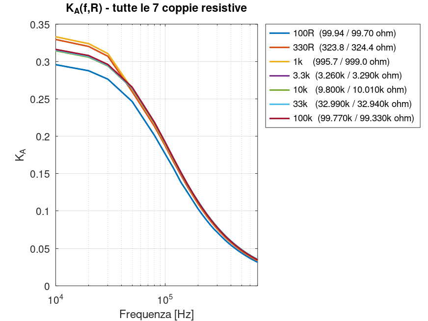 Rapporto tra tensione differenziale misurata sul ramo di iniezione e Vgen per la configurazione A, riportato per tutte le sette coppie resistive.
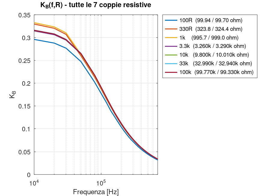
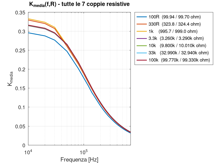
The three graphs show a fairly clear pattern. At lower frequencies, the curves for the different resistance values are more widely separated, while they progressively converge as frequency increases. The dependence on DUT impedance therefore appears stronger in the lower part of the band, whereas at higher frequencies the injection-transfer behavior becomes much more similar among the different resistive configurations.
It is also interesting to note that KA and KB show very similar trends and that their average retains the same overall structure. This makes K_avg a particularly useful quantity for continuing the analysis, because it reduces the weight of differences associated with A/B orientation and allows the common behavior of the system to be examined more directly.
For the moment, I do not consider this ratio a direct measurement of DUT impedance. The goal is to determine whether there is a sufficiently regular relationship between Vgen, the actual injected voltage, frequency, and load impedance that could later be used as additional information when characterizing both the DUT and the GX LII-2 itself.
It should also be remembered that the curves shown here were not obtained with Vgen held constant throughout the sweep: the generator amplitude was changed as a function of frequency to maintain an adequate signal level. Frequency and Vgen are therefore not yet experimentally separated variables in this analysis of K.
It is important to distinguish this analysis from the tests performed in recent days on the influence of Vgen on the Bode plot. In those tests I experimentally verified that, as long as the system remains in its linear region, using a fixed Vgen or varying it to improve the signal level does not significantly change the final magnitude and phase result.
The parameter K introduced here is a different quantity: it directly describes the ratio between the differential voltage across the injection branch and the voltage set on the generator. Its possible independence from Vgen has not yet been experimentally verified.
The available measurements show a clear dependence on frequency and some separation among the different impedances, but at this stage I cannot yet assume that:
rather than, more generally,
Separating these dependencies will therefore require a dedicated test, keeping frequency and divider constant while varying only Vgen. This does not call into question the previous verification that the Bode plot is independent of Vgen: it concerns only the new parameter K and its possible use as additional information about the behavior of the injection circuit and, potentially, DUT impedance.
It is therefore perfectly possible to have, at the same time:
independent of VGEN, but:
Overall results of the resistive campaign
With the campaign on the seven resistive dividers completed, I can finally compare all configurations from 100 Ω to 100 kΩ in the same way.
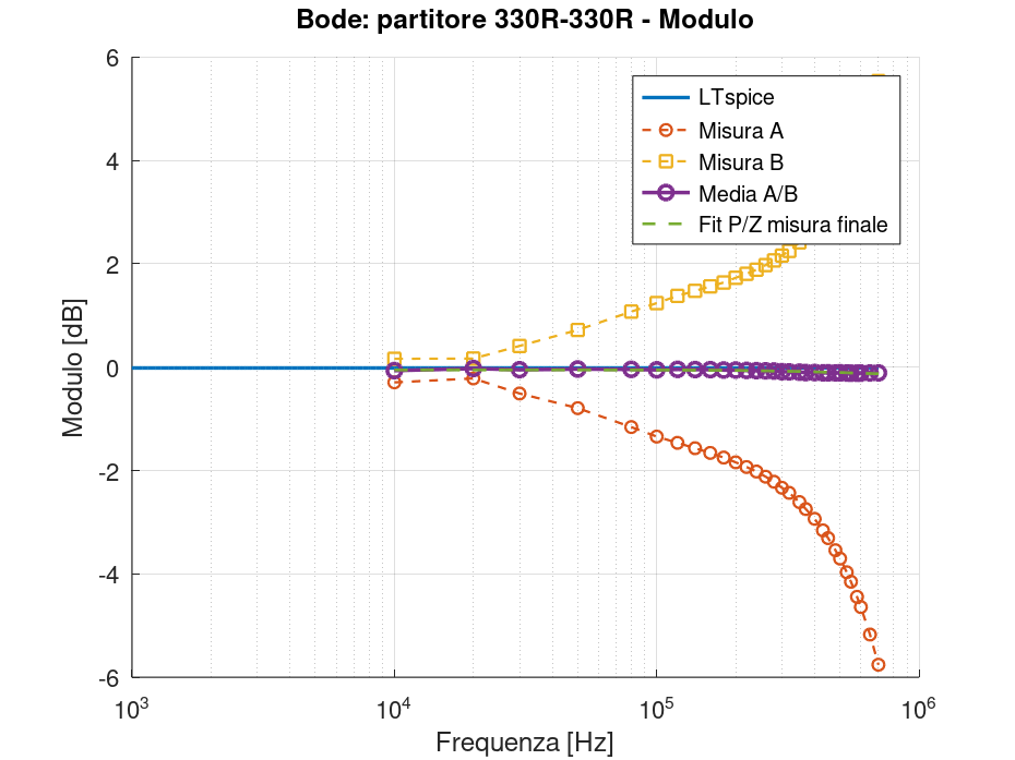
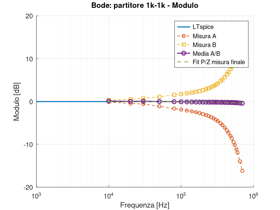
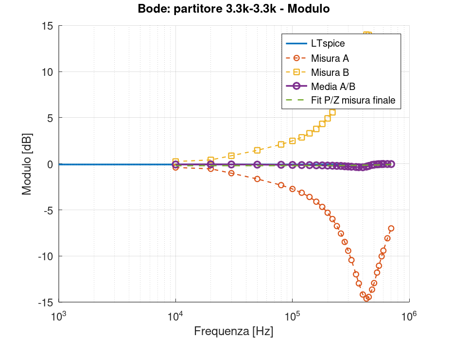
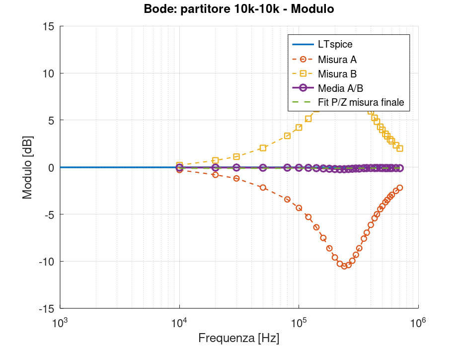
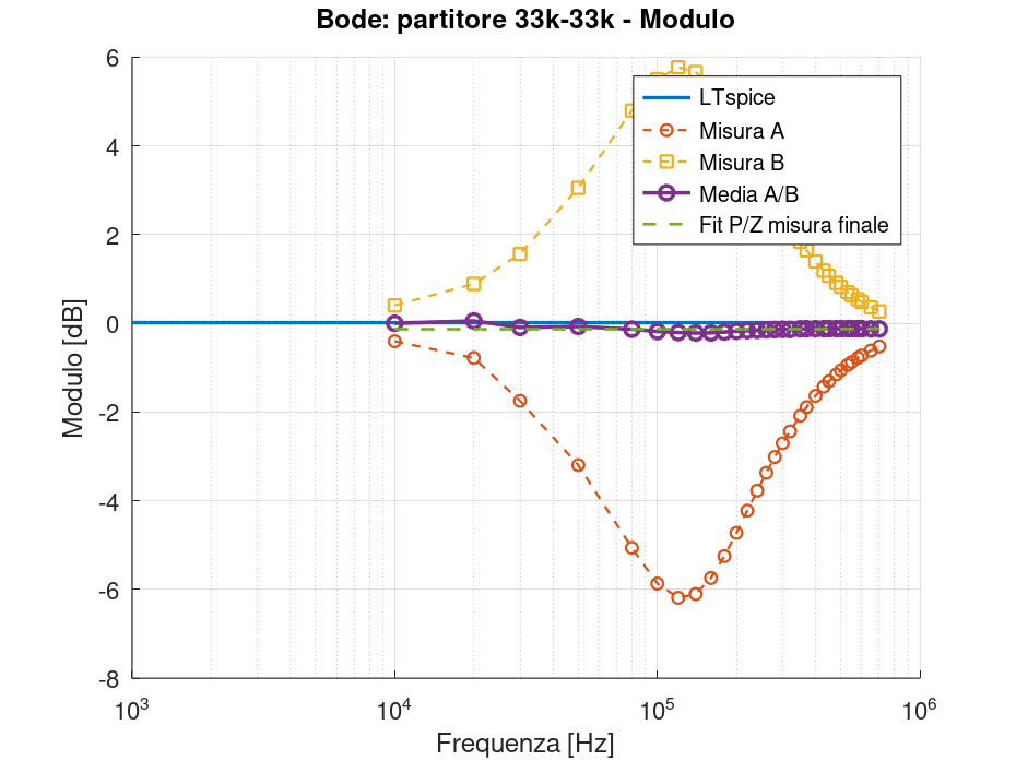
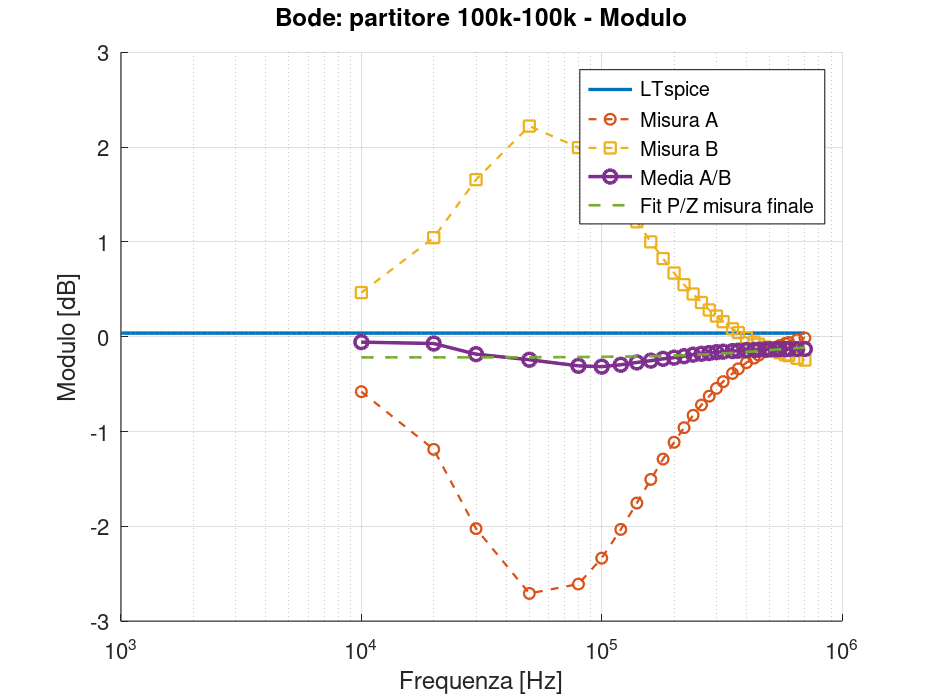
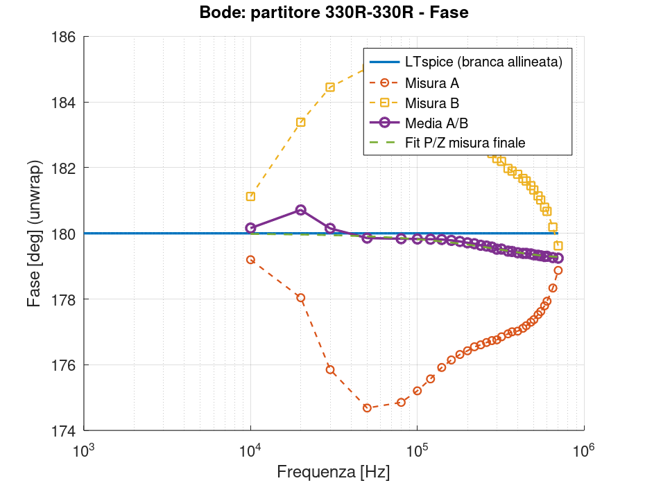
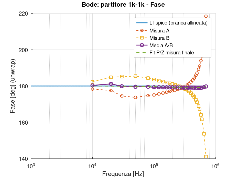
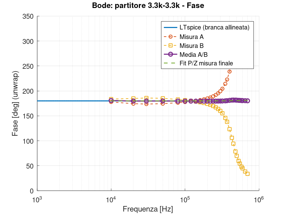
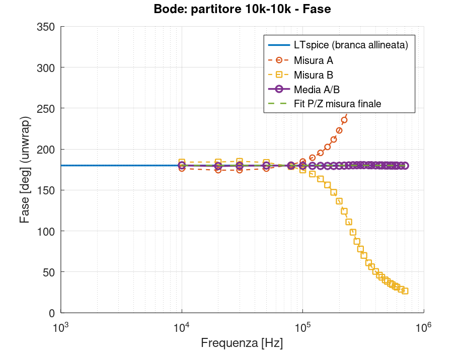
The following graphs show, for each divider, the magnitude and phase obtained in the two A and B configurations, the result of their combination, and the reference obtained from the LTspice simulation.
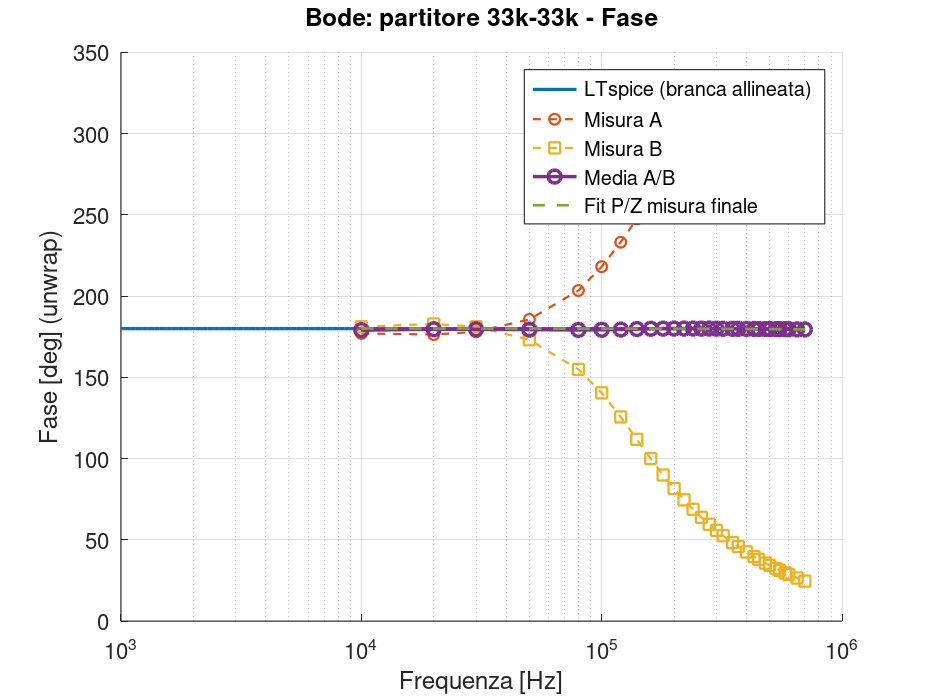
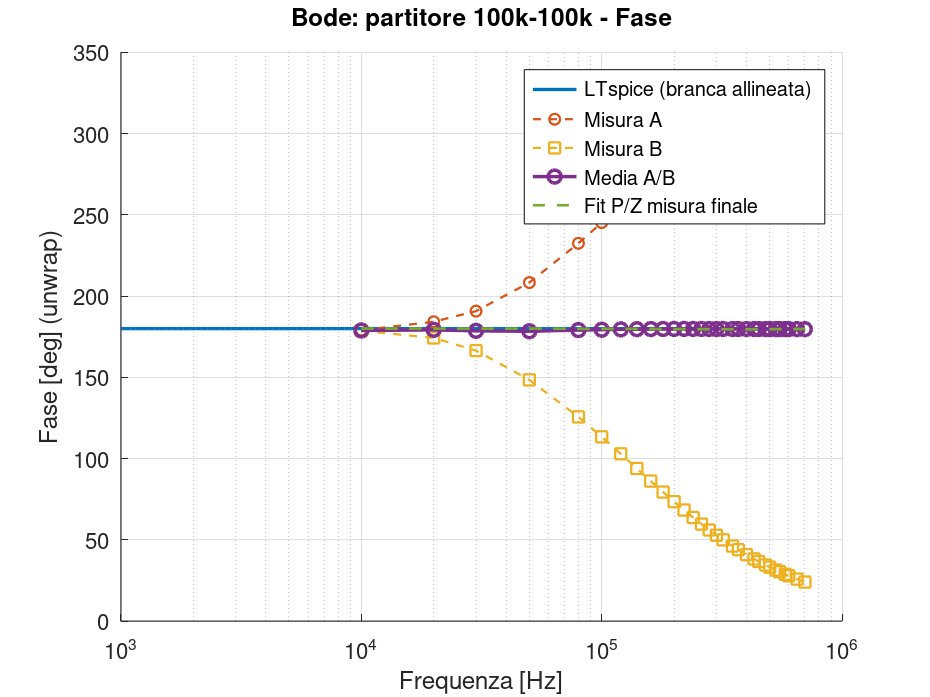
An important result is already evident from a first visual inspection: the final measurement obtained from the A/B combination is much more robust than the individual A and B measurements. The latter can diverge substantially as frequency and impedance increase, while the combined result remains generally close to the behavior predicted by the simulation.
This does not, of course, mean that the system is now fully characterized. This campaign concerns only resistive impedances and does not yet allow the same conclusions to be extended to DUTs whose impedance at the injection point has a significant reactive component. This is one of the reasons why the calibration bench also includes a capacitive section, which I will use in a later phase.
For the conditions explored so far, however, the results are beginning to show that the A/B method can keep the final measurement sufficiently stable even when the two acquisitions, considered separately, become strongly dependent on secondary-winding orientation.
Magnitude
In the first gallery I collected the magnitude plots for all seven resistive pairs, ordered from 100 Ω to 100 kΩ. This makes it possible to follow directly how the separation between A and B evolves with impedance and frequency and, above all, to compare it with the behavior of the compensated final measurement.
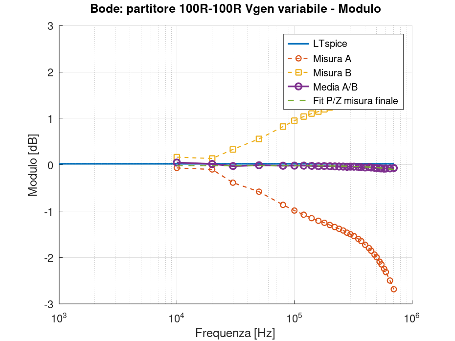 Modulo della funzione di trasferimento per il partitore resistivo 100 Ω–100 Ω. Le misure A e B si separano progressivamente con la frequenza, mentre la combinazione A/B rimane molto vicina al riferimento LTspice.
Phase
The second gallery shows the phase plots in the same order. Here too, the main point is to compare the evolution of configurations A and B with the result obtained after combining them.
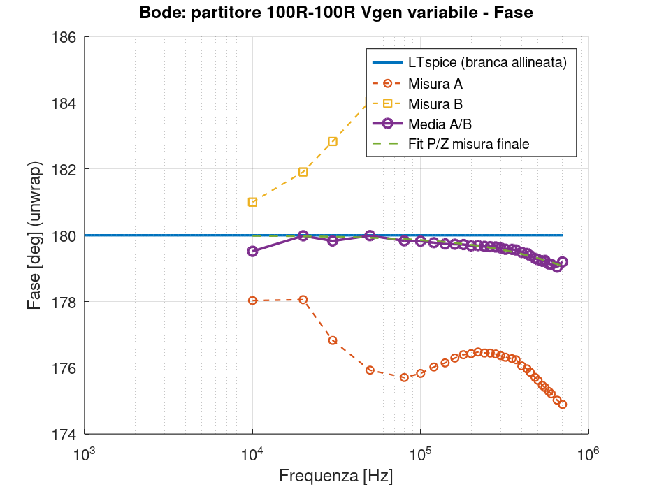 Fase misurata sul partitore 100 Ω–100 Ω. L’inversione A/B produce deviazioni opposte, mentre la fase mediata rimane prossima al comportamento previsto dalla simulazione.
Acquisition diagnostics
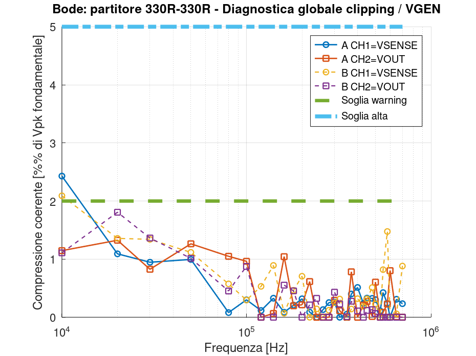
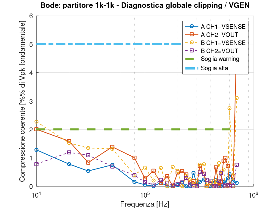
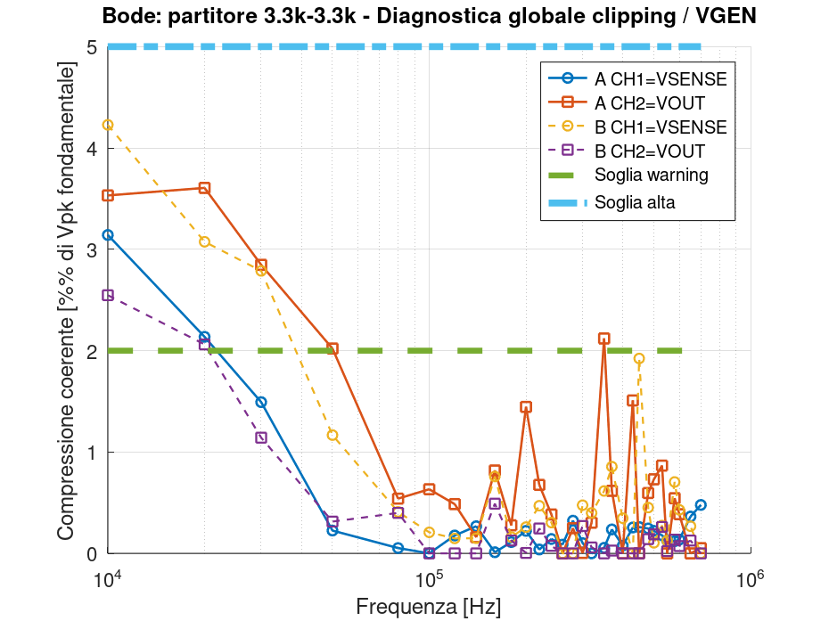
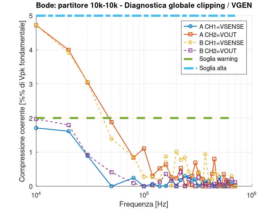
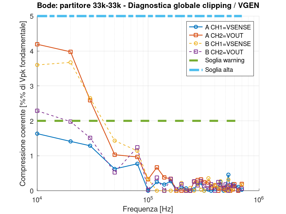
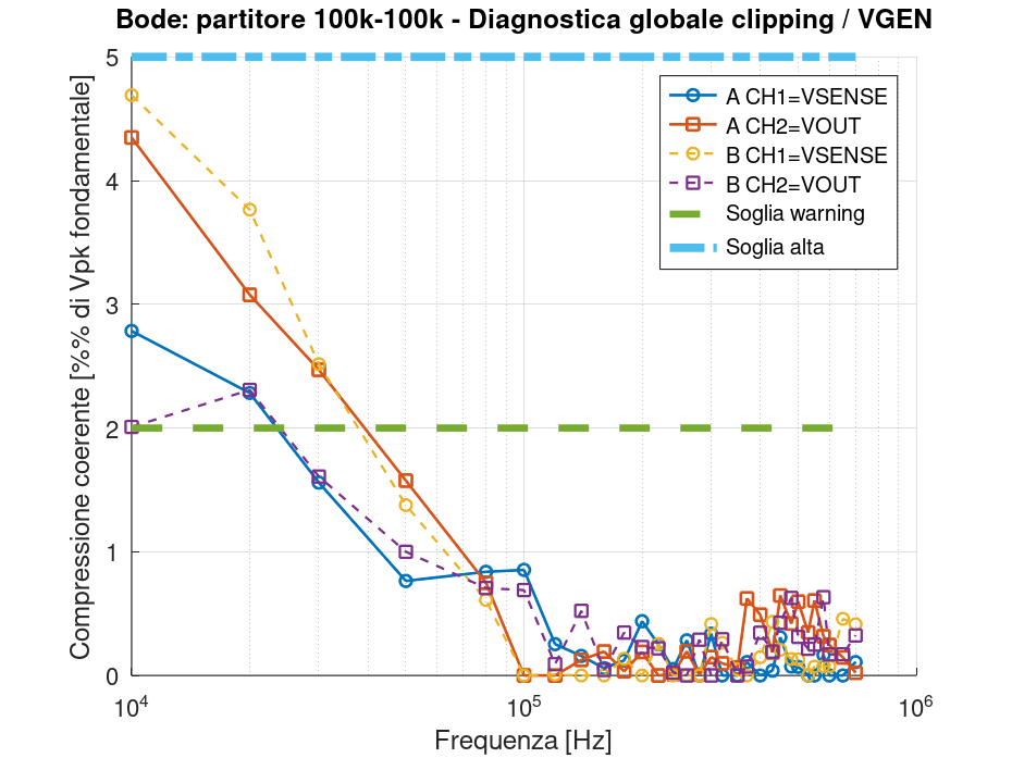
To complete the results, I also include the plots produced by the Octave script for coherent waveform-deformation diagnostics. These plots do not directly enter the Bode calculation, but provide an additional check on acquisition quality and on the possible presence of compression or systematic waveform deformation.
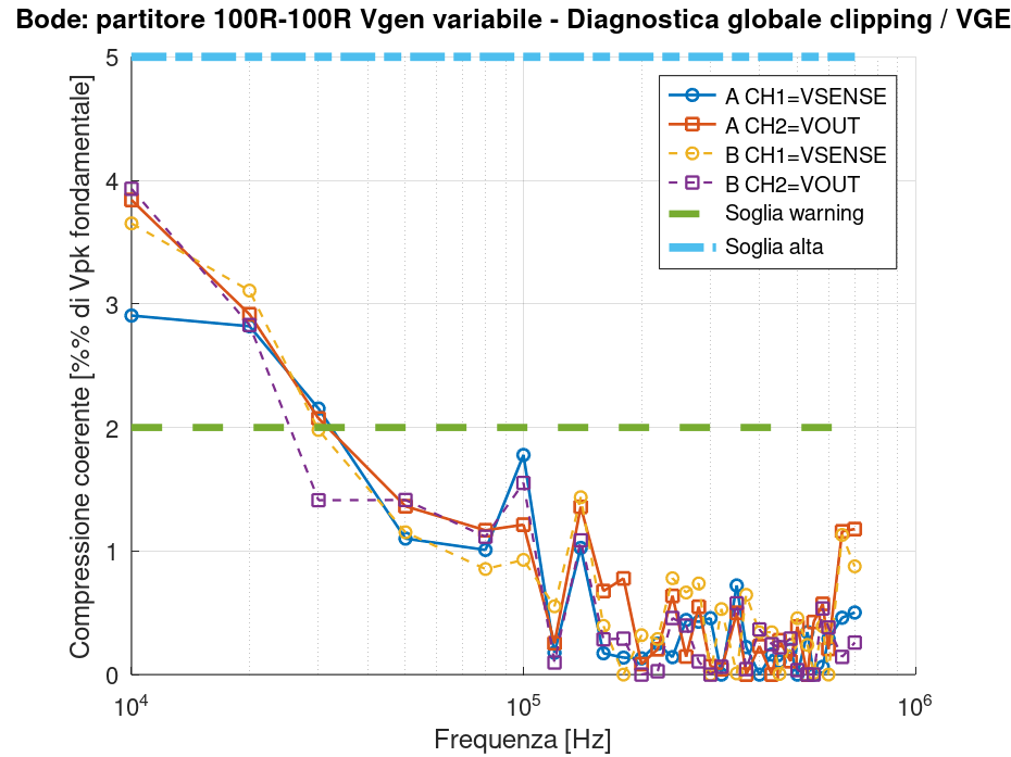 Diagnostica della deformazione coerente delle acquisizioni A e B per il partitore 100 Ω–100 Ω. Il controllo è utilizzato come indicatore complementare della qualità delle acquisizioni.
To avoid judging the effectiveness of A/B compensation only by visual inspection, I also summarized the deviation of the final measurement from the LTspice model over the entire acquired bandwidth. For each divider, the table reports the mean absolute error and the maximum deviation observed across the 30 measurement points.
| Divider | mean |ΔM| [dB] | max |ΔM| [dB] | mean |Δφ| [°] | max |Δφ| [°] |
|---|---|---|---|---|
| 100 Ω | 0.065 | 0.104 | 0.452 | 0.963 |
| 330 Ω | 0.064 | 0.101 | 0.450 | 0.754 |
| 1 kΩ | 0.159 | 0.397 | 0.757 | 1.163 |
| 3.3 kΩ | 0.106 | 0.294 | 0.645 | 1.684 |
| 10 kΩ | 0.092 | 0.202 | 0.262 | 0.737 |
| 33 kΩ | 0.147 | 0.233 | 0.300 | 0.924 |
| 100 kΩ | 0.215 | 0.354 | 0.438 | 1.615 |
Across all seven series, the mean absolute magnitude error remains between about 0.064 and 0.215 dB, while the phase error remains between about 0.26° and 0.76°. The maximum deviations observed over the entire campaign also remain below about 0.40 dB in magnitude and 1.7° in phase. These figures therefore provide a quantitative measure of what is already evident in the plots: the deviations of the individual A and B measurements can be very large, but the residual after combining them remains much smaller.
Revisiting the 33 kΩ case
These results also lead me to revisit a point made in the first article in the series, when characterization was still at an early stage.
For the 33 kΩ divider I wrote:
Here too, reversing the secondary highlights an asymmetric component, but the A/B average no longer matches the response predicted by the simulation. A component of the error therefore remains in both secondary orientations and cannot be eliminated by reversal.
I then continued by observing that:
The tests indicate that there are at least two different contributions: one associated with transformer asymmetry, which changes sign when the secondary is reversed and can therefore be greatly reduced by combining A and B, and a second contribution common to both measurements, which becomes important under certain impedance conditions.
That description accurately reflected what emerged from the first available acquisitions. The complete resistive campaign now makes it possible, however, to put that initial interpretation into better perspective.
The large deviation of the A/B average observed at the time with the 33 kΩ divider does not reappear with the same magnitude in the new measurements. On the contrary, the current plots show that even when the individual A and B configurations begin to diverge strongly, their combination generally remains much closer to the LTspice reference.
This does not mean that every error common to the two configurations has disappeared. A residual after A/B compensation is still present and, as I will examine more closely shortly, has its own dependence on frequency and impedance. What has changed compared with the first observations is mainly its magnitude, which is considerably smaller than those initial 33 kΩ tests suggested.
I cannot retrospectively determine which single factor produced the deviation observed at that stage. The initial measurements were mainly exploratory, and the experimental setup was not yet being managed with the level of care achieved during this campaign.
During the tests it became clear just how sensitive these measurements are to bench conditions. The signals at OUT and SENSE can be only a few tens of millivolts and, under these conditions, ambient noise, common-mode currents, cable routing, connection quality, and other elements of the measurement chain can become comparable with the useful signal.
For the current campaign I therefore tried to reduce these error sources systematically, paying greater attention to wiring and grounding, eliminating unnecessary interference sources from the bench, using ferrites on the connections, and relying on Octave’s fundamental-component fit to extract magnitude and phase.
The problem encountered with the intermittent BNC connector was also a very concrete example of how an apparently minor defect can cause significant changes in acquisitions of this type.
I therefore do not regard the initial 33 kΩ result simply as a “bad measurement.” It was instead a useful step in the characterization because it showed how important it is to check the entire experimental chain before attributing a structure observed in the data to the DUT or the transformer.
In light of the current campaign, I can therefore say that, at least for the resistive loads explored, the A/B system is performing better than those early measurements suggested.
A residual of the combined measurement relative to the reference nevertheless remains, and its structure deserves closer examination.
A/B compensation and residual measurement error
The plots obtained for the seven resistive pairs clearly show a behavior already observed in the first tests: as frequency increases, the measurements made in the A and B configurations can move far away from the LTspice reference. The deviations, however, occur predominantly in opposite directions.
For this reason I do not interpret this component as an error common to both measurements, but as an error dependent on transformer orientation, essentially antisymmetric with respect to A/B reversal.
A very simple model, which I do not consider exact but which describes qualitatively what I observe quite well, is:
where E schematically represents the error component that changes reciprocally when the secondary terminals are reversed.
In this ideal model, combining the two measurements gives:
In my case the combination is performed in the logarithmic domain for magnitude and after alignment of the phase branches; the meaning is nevertheless equivalent to a geometric mean of the linear quantities.
A particularly clear example can already be seen in the 100 Ω series: at 700 kHz measurement A reaches about −2.60 dB, while B is about +2.51 dB; after A/B combination the result returns to about −0.044 dB, with a phase of about 179.45°.
The A/B average is therefore not simply reducing random noise: the results are highly consistent with cancellation of a component that is nearly reciprocal with respect to transformer reversal.
What remains after this compensation is the quantity that, at least for now, I want to define as the common residual of the measurement relative to the reference. This residual cannot automatically be attributed to either the transformer or the DUT. If I represent it schematically as an overall factor in the measurement chain, I can imagine something like:
This expression is deliberately qualitative: its main purpose is to emphasize that the observed residual belongs to the entire DUT + measurement-system chain, and not necessarily to a single element.
The first practical conclusion from the resistive campaign is nevertheless positive. Under the conditions characterized so far, A/B compensation keeps the residual small enough for me to consider the GX LII-2 already usable, at least as a first approximation, for DUTs in which the impedance seen from the injection point is predominantly resistive and falls within the explored range.
This conclusion cannot yet be extended to impedances with a significant reactive component. This is precisely one of the reasons why the calibration bench also includes a capacitive section: I will have to verify whether the same cancellation capability is retained when the impedance becomes complex.
Another interesting aspect is that the residual of the A/B measurement does not appear to behave like a simple calibration constant. The plots show dependencies on both frequency and impedance. In some regions, especially at lower impedances and below about 100 kHz, small non-monotonic structures are also visible. At present I cannot determine whether these are actual resonances: they could result from interactions among the transformer, parasitic capacitances and inductances, Rinj, wiring and, more generally, the measurement fixture, as well as the probes and acquisition chain.
In the future I would therefore like to study the residual not only as an error to be corrected, but also as a possible observable quantity capable of providing information about both the DUT and the behavior of the measurement system itself. I will not try to build such a model yet: this first campaign is intentionally exploratory.
For the moment, the practical result is simpler: the individual A and B measurements can become strongly orientation-dependent, while their combination remains much more stable and close to the simulated reference.
Global FFT analysis of the A/B acquisitions
As a final check on the resistive campaign, I also used the acquisitions already available for a broader spectral analysis. The goal was not to produce a separate FFT for every CSV: with dozens of frequencies and two A/B configurations for each divider, this would have produced hundreds of spectra that were difficult to compare. I therefore chose to build a GNU Octave script that automatically summarized the spectral content of the entire campaign for each divider, while still keeping configurations A and B separate.
For each CSV, the script knows the test frequency from the same association file used for Bode processing. Both channels are analyzed, with CH1 = VSENSE and CH2 = VOUT; the final summary retains the channel on which a given component reached its highest amplitude.
The important point is that the fundamental is not removed simply by zeroing the nearest FFT bin. Instead, for each acquisition a time-domain fit is performed
and the FFT is then performed on the residual
In this way, both the DC component and the fundamental at the exact frequency set for that measurement are removed, greatly reducing the risk that the fundamental and its spectral leakage dominate the residual spectrum. The harmonics 2f0, 3f0, etc. are intentionally left in place and can therefore be identified by the analysis.
Before the FFT, a Hann window is applied and its coherent gain is compensated; a single-sided spectrum expressed in Vpk is then obtained. To compare all acquisitions directly, the script also selects the most common Increment value and a common number of samples so that the spectra share the same frequency grid. In the typical case of these acquisitions, with Δt = 4 ns and 300000 samples, this gives 250 MS/s, a duration of about 1.2 ms, a resolution of about 833.3 Hz per bin, and a Nyquist frequency of 125 MHz.
The next step is perhaps the most distinctive aspect of this analysis. The spectra from the different acquisitions are not averaged. Instead, for each bin the maximum amplitude encountered over the entire campaign is retained:
This produces two maximum envelopes, one for A and one for B. These plots do not represent the system’s “average spectrum”; rather, they answer the question: which spectral lines managed to become most prominent at least once during the entire campaign?
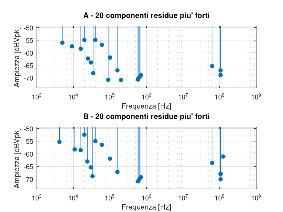
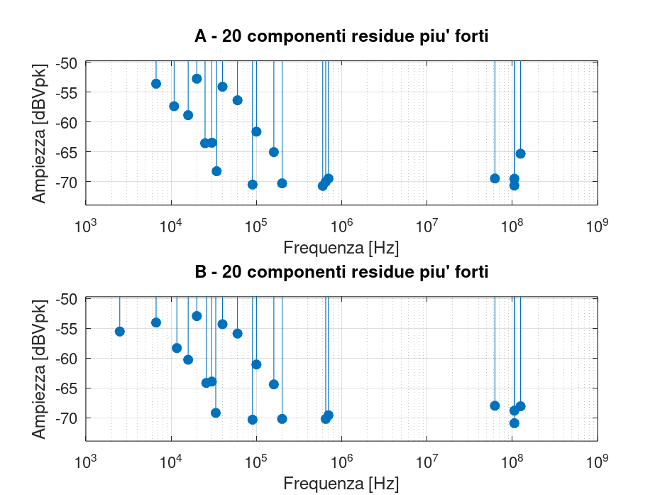
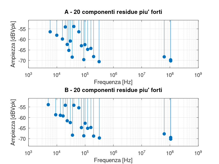
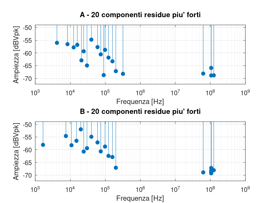
The 20 strongest local maxima are then selected from the envelopes for A and B. For each maximum, the CSV files retain frequency, amplitude in Vpk and dBVpk, channel, the test frequency of the CSV that produced it, source filename, and classification. This keeps the graph compact while still allowing every peak to be traced back to the measurement from which it originated.
Some maxima in the first few kilohertz also appear in the lowest part of the spectrum. With the approximately 1.2 ms record duration used in these acquisitions, any 50 or 100 Hz components cannot be resolved as separate spectral lines: they appear mainly as slow variations within the record and can contribute to leakage in the first bins. For this reason, I do not currently assign a specific origin to the structures observed in this region.
A significant fraction of the peaks consists of harmonics
Analyzing the files fft_top_A.csv and fft_top_B.csv for all seven resistive dividers — 100 Ω, 330 Ω, 1 kΩ, 3.3 kΩ, 10 kΩ, 33 kΩ, and 100 kΩ — makes this characteristic particularly clear.
Considering all 280 peaks selected by the script, that is, 20 for each A/B configuration of the seven dividers, 100 are low-order harmonics identified directly from their relationship to the test frequency. Specifically:
81 second harmonics, 18 third harmonics, and one fourth harmonic.
This is therefore more than one third of the entire set of selected maxima, rather than a handful of isolated coincidences.
Some relationships appear repeatedly across different dividers and orientations. For example, 40 kHz in the 20 kHz test, 60 kHz in the 30 kHz test, 100 kHz in the 50 kHz test, 160 kHz in the 80 kHz test, and 200 kHz in the 100 kHz test are all 2f0 components.
Similarly, 3f0 components appear, such as 30 kHz in the 10 kHz test and 90 kHz in the 30 kHz test. The campaign also contains one component classified as a fourth harmonic, i.e. 4f0.
This provides a useful internal check of the entire procedure. After intentionally removing the fundamental, the script recovers a large number of the components expected to remain when the waveform is not perfectly sinusoidal. The fundamental is subtracted by time-domain fitting, while 2f0, 3f0, and higher harmonics are deliberately left in the residual.
The observed harmonics are therefore not simply an artifact of using maximum envelopes: many of the selected lines retain a precise and repeatable relationship with the excitation frequency.
It should also be remembered that only the 20 strongest local maxima are shown for each A or B campaign. The absence of a particular harmonic from the ranking therefore does not mean that it is absent from the spectrum; it only means that, in the global envelope for that series, at least twenty structures reached a greater amplitude. The script also retains the complete aggregated spectrum, bin by bin.
Components that do not follow the test frequency
Alongside the harmonics, however, a second group of signals appears with completely different characteristics.
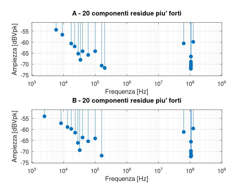
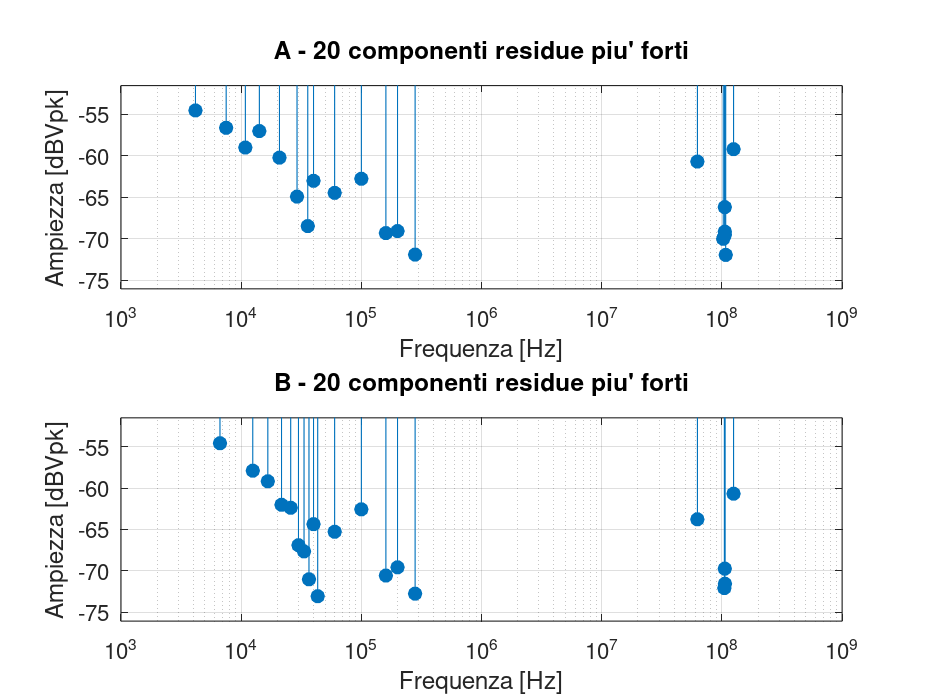
The line at 62.5 MHz is particularly evident: it appears among the selected maxima in both A and B for all seven dividers analyzed.
Across the entire campaign, its maximum amplitude lies approximately between 0.34 and 0.98 mVpk, corresponding to about −69.5 to −60.2 dBVpk.
A structure around 105.7 MHz is also extremely recurrent and can be observed across all the different impedances and in both A and B configurations. In this case it is more accurate to describe it as a group of spectral lines, because the script often selects several closely spaced maxima in the same region. The selected peak amplitudes are typically around −72 to −66 dBVpk.
A component close to 125 MHz appears in many, though not all, of the A/B rankings. The value is generally that of the bin immediately below 125 MHz, which is entirely consistent with the discrete nature of the FFT grid.
For two of these structures, the relationship with the sampling rate is particularly clear:
and
With fs = 250 MS/s, the second frequency therefore coincides with the Nyquist frequency.
The feature I find most interesting is not simply the absolute frequency values, but their recurrence across seven different impedances, two transformer orientations, and many excitation frequencies.
Unlike the low-order harmonics, these lines do not shift with f0.
For this reason, I currently consider it plausible that at least some of these components belong to the acquisition chain rather than to the resistive DUT or the intentionally injected signal. Possible contributors include clocks, ADC operation, sampling architecture, internal digital processing, aliases, or other elements of the instrumentation.
The region around 105.7 MHz does not show an equally simple relationship with fs, so the data currently available do not allow a specific origin to be assigned to it.
This intentionally remains an experimental hypothesis, not a definitive identification of the source.
Caution when interpreting the automatic classification
There is one final important detail in interpreting the CSV files.
The script checks whether the frequency of each maximum is compatible with an integer multiple of the test frequency of the CSV from which that maximum originates. This criterion works very well for low-order harmonics such as 2f0, 3f0, or 4f0, but it can produce purely mathematical coincidences when the frequency ratio becomes very large.
I therefore do not regard these labels as proof that a component is harmonic in origin. To distinguish physically meaningful harmonics of the test signal from recurrent spectral lines, the harmonic order, the test frequency of the source file, and above all whether the line frequency follows f0 or remains essentially fixed as the measurement changes must all be considered together.
This is precisely what makes the many 2f0, 3f0, and 4f0 components much more significant: in those cases, the line frequency actually follows the excitation frequency.
What this analysis says about acquisition quality
This processing therefore adds another level to the characterization.
On one hand, it separates the intentional fundamental and reveals numerous harmonics consistent with the test signal, providing an independent check on the non-sinusoidal content of the acquisitions.
On the other hand, as the amplitude decreases further, components begin to emerge that do not follow the excitation frequency and instead appear to belong to the instrumentation or, more generally, to the acquisition chain.
The observed high-frequency lines range from a few hundred microvolts up to about 1 mVpk. The fact that structures of this amplitude are distinguishable and recurrent across all seven resistive campaigns does not, of course, demonstrate the absolute accuracy of the bench, but it does indicate that acquisition stability, signal-to-noise ratio, and numerical processing are sufficient to reveal phenomena much smaller than the fundamental used for the Bode measurement.
This is also an interesting methodological result: after working to reduce noise, connection problems, and common-mode interference, the acquisitions are consistent enough not only to derive magnitude and phase, but also to observe the residual spectral structure of the measurement.
The files produced by the script also retain both the peak rankings and the full aggregated envelope bin by bin; the PNG files are therefore only a compact representation of data that remain available for numerical analysis.
FFT analysis gallery
The following plots collect the results of the global FFT analysis for all seven resistive pairs, from 100 Ω to 100 kΩ. For each divider, the upper panel shows the 20 highest-amplitude residual components identified in campaign A, while the lower panel shows the corresponding result for campaign B. The intentional fundamental was removed before the FFT, so the plots contain harmonics, spurs, and other residual components that emerged from the full set of acquisitions.
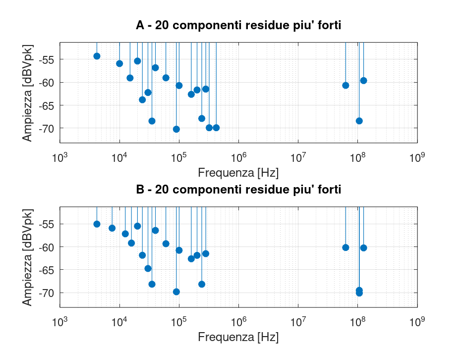 Analisi FFT globale del partitore da 100 Ω. Sono riportate le 20 componenti residue di maggiore ampiezza emerse nelle campagne A e B dopo la sottrazione della fondamentale intenzionale.
The Octave script and guide can be downloaded below; unfortunately, the ZIP archive containing all the CSV files is too large to upload here.
Conclusions
With this spectral analysis, I consider the first systematic GX LII-2 characterization campaign on resistive dividers complete.
The measurements made it possible to verify the robustness of A/B compensation, quantify the residual relative to the simulation, begin studying the relationship between Vgen and the actual injected voltage, and finally use the same acquisitions to examine residual spectral content beyond the fundamental.
The global FFT revealed a particularly interesting distinction: on one hand, numerous low-order harmonics appear that directly follow the test frequency; on the other, recurrent high-frequency lines emerge that are largely independent of the resistive DUT and f0, potentially providing a signature of the acquisition chain.
I do not consider these results a definitive calibration of the instrument, but rather a first experimental characterization broad enough to begin distinguishing what belongs to the measurement, what depends on the injection system, and what may belong to the instrumentation used to observe it.
In the next few days I will perform measurements with the capacitive bench.