

Calculation and preview
The calculation uses the rows marked with dots in the Selected column. Choose the curve type, method and resolution, then press Preview.
Mode
- 2d
- It is the initial setting. For an ordinary curve the Builder calculates Y according to X after ordering points for X increasing. X must assume distinct values. You can combine 2d, arc_length and geometric order revised for a sequence planar contour. In that case, X and Y are calculated according to the route.
- 3d
- Calculate a parametric line in space. Choose X, Y, Z and a type of Parameter, then load the rows. A point surface can produce a path in their order. To reconstruct a surface, a flow dedicated to the surfaces is needed.
If you switch between 2D and 3D after loading rows, use Restart sources, check the axes and load the rows again. The Builder reads the required coordinates when you use Add source rows.
Parameter
- variable
- This is the default. In 3d, select the t column before loading the rows. In the standard workflow, Curve Builder sorts by increasing t and evaluates X(t), Y(t) and Z(t) separately. X, Y and Z can have different units. Check that t values are distinct and that increasing t represents the acquisition order. In ordinary 2d, X is the independent variable.
- arc_length
- In 3d, load X, Y and Z in the same unit. The parameter starts at zero and accumulates the distance between consecutive points. The unit of t is the common axis unit. With Auto-order off, the Builder uses the loading order of the marked points. Consecutive coincident points create a zero-length segment and must be excluded or reloaded. In 2d, the calculation remains Y(X) until you enable and accept a proposed geometric order, which requires the same unit for X and Y.
Method
Interpolation methods reproduce the data at the nodes. Fits estimate a trend from the selected data and can have residuals at the nodes. The method applies to each dependent coordinate. All methods evaluate within the range covered by the rows used in the calculation.
| Method | How to use it and what to check |
|---|---|
| nearest | Select at least 2 points to use the value of the nearest node. The preview shows values that repeat over intervals, with jumps between measured values. The plotted line connects the displayed samples. |
| linear | This is the default. Select at least 2 points to connect consecutive values with straight segments. Use the preview to check the slopes between nodes and the corners at the nodes. |
| cubic | Select at least 3 points for piecewise cubic interpolation. In the tested version it behaves like pchip on these data. Check that the curve passes through the nodes and inspect the transitions. |
| spline | Select at least 3 points for a cubic spline. It is suitable to show smooth transitions. Check any fluctuations or values beyond the local extremes, especially between distant knots or near the extremes of the curve. |
| pchip | Select at least 3 points for the piecewise cubic Hermite interpolant, which preserves local shape. Use it to preserve monotonic trends in sections of the data. Check the nodes and transitions in the plot. |
| line | Select at least 2 points with distinct independent coordinates to fit a straight line by least squares. Use the diagnostics to assess the overall trend. The Polynomial degree setting has no effect on this fit. |
| polynomial | Select at least 2 points and set Polynomial degree. The preview evaluates the least-squares polynomial fit at the target samples. Choose a degree appropriate to the phenomenon and check the plot and reported residuals. A high degree can introduce oscillations. |
Polynomial degree
Write an integer. The initial value is 2. With polynomial you can use 0 for a constant model, 1 for a first degree model or higher degrees up to one in less than the number of marked points. The Polynomial degree must be between 0 and one less than the selected point count. message requires you to correct the field or select multiple points. In other methods, the field remains visible.
Target samples
Insert a whole from 2 to 100000. The initial value is 101. The grid includes that number of uniform samples between the two extremes and integrates the coordinates of the original knots, eliminating the doubles. The actual count can then exceed the one required. With multiple samples the drawing traits appear more dense and the table published can grow. If Target sample count must be 2–100000. appears, correct the number.
Preview
Press Preview after marking at least two points. If Auto-order is on and you have not reviewed the proposed order, the button opens Original and proposed processing order. Accept the proposal or return to the normal order, then press Preview again. Preview: … target points from … selected source rows. reports the generated samples and the rows actually used.
If you see Select at least two source points., load and mark the rows. If the independent coordinate is not strictly increasing, check for repeated X or t values, duplicate loads and zero-length segments. After changing the method, degree, sample count, dimension or parameter, run Preview again even if an earlier plot is still visible. If any source rows come from a changed schema, reload those sources before retrying.
NUMERIC_API preview values (first 500 shown)
Scroll the bottom table to read the first 500 rows of the result. After Clear selection or a Preview attempt that returns an error, the table can retain the previous values. Before reading them, check that the status bar brings a successful Preview on the current selection. Use state count to know the total processed and the Dataset published to access all samples.
| Column | Value displayed |
|---|---|
| X or t | In ordinary 2D mode, this is the target X value. In 3D or in a parametric planar contour, it is t in the unit of the t variable or of the cumulative path length. |
| X | X coordinate calculated in a parametric path. In 2D ordinary read the ascissa in the first column. |
| Y | Measured or coordinated Y interpolated or estimated. |
| Z | Z coordinate calculated in 3D. In 2D the column remains empty. |
Curve Builder Plot Dataset preview
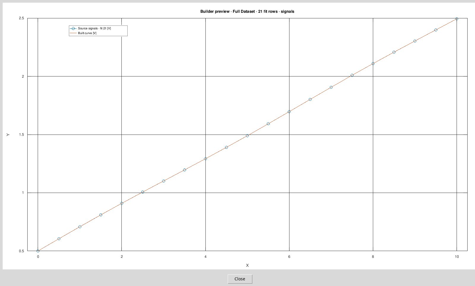
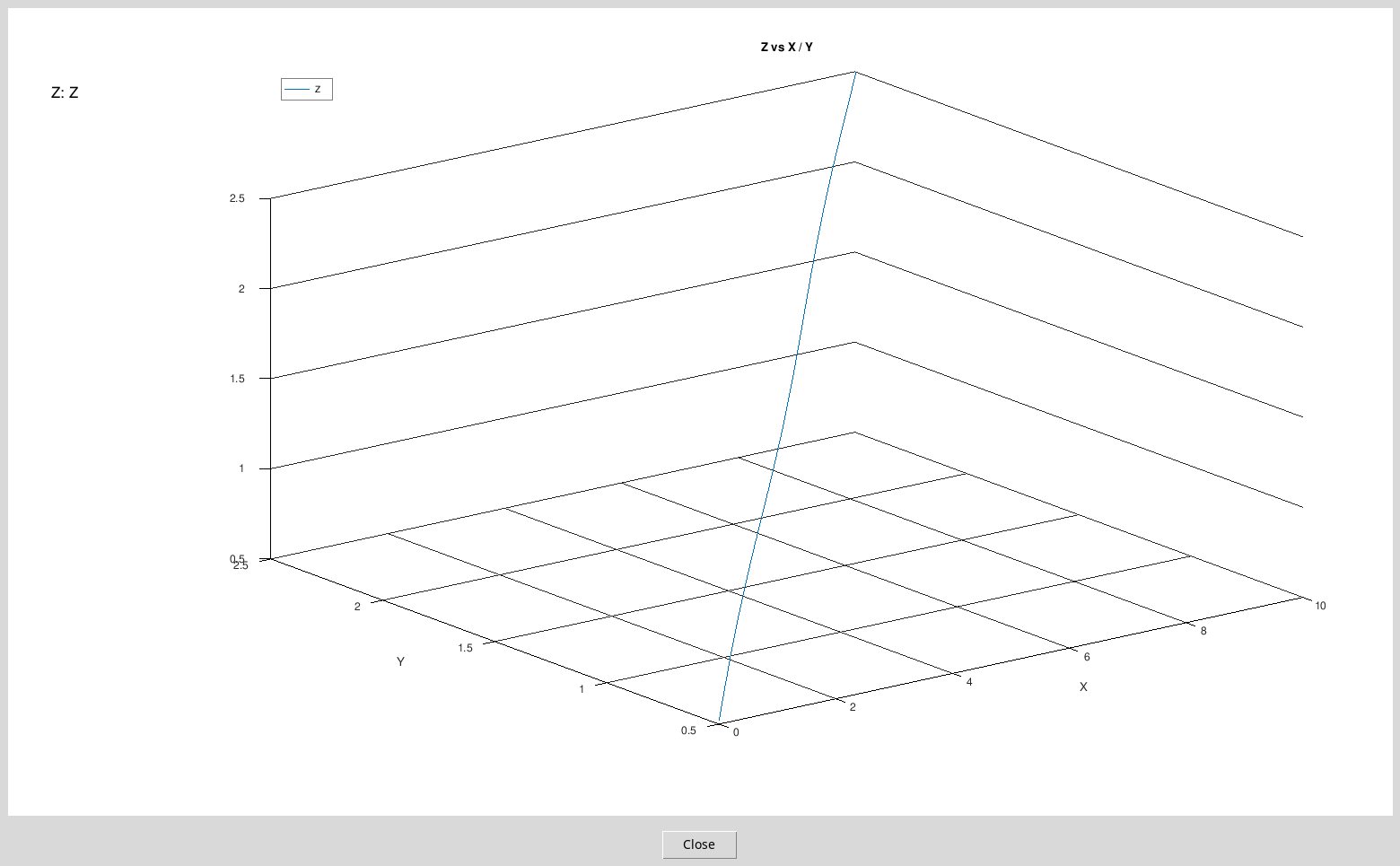
The temporary plot window opens with Preview. In 2d compares the Built curve line with sources. The title shows the context shown, the count of the points used and the Dataset. In 3d the image shows the parametric line built along X, Y and Z. To rotate the 3D representation, use the scene that is opened after publication with the active overlay option.
Close or the closing control of the plot window closes the image. The processed values remain available for publication until the Preview remains valid.
Diagnostics for line and polynomial
| Metric | How to read it |
|---|---|
| Observations | Number of observations used to adapt each response. Check that matches the number of expected rows. |
| Root mean squared residual | RMSE is the root mean square of the residuals, expressed in the response unit. It indicates the size of the residuals at the points used for the fit. |
| R squared | R2, dimensionless. It sums up the adaptation to the variability of the response. With constant response it can appear undefined because the denominator is zero. Undefined indicates a non-interpretable statistics in that case. |
A parametric fit reports separate diagnostics for X, Y and, in 3D, Z as functions of the parameter. RMSE is expressed in the unit of each coordinate. For coefficients stored in metadata, the line fit uses intercept and slope, while the polynomial fit orders coefficients by descending powers. The fitted curve and statistics use the selected rows. The Builder does not estimate confidence intervals without a noise model.