

Guided scientific operations
Set operands and prerequisites, run guided GX-TXT operations, and apply a captured result field to the worksheet.
Find a function and distinguish the execution modes
Open Functions, from the toolbar button or with F3. Type a name or a term from the description in the search field. Select an entry to read signature, arguments, form, units, result fields, modes and providers. The guided catalog collects the visible identifiers and points to the families.
- formula
- You can type the function in the cell or use Insert formula to start the expression. The input and output types are those exposed for the operation. A vector calculation can extend over several cells.
- guided
- Fill in the editor in the panel. Use guided operations for typed contracts, options, models and structured results. Some names also have a compatible form for use in an expression, such as
field(numeric.statistics(...),"mean"). - unavailable
- The panel shows the reason.
numeric.configure_fft_threadsconfigures a process,numeric.foundationidentifies the group with named actions andsignal.statistical_contractdescribes a contract. Find the relevant calculation operation in the catalog.
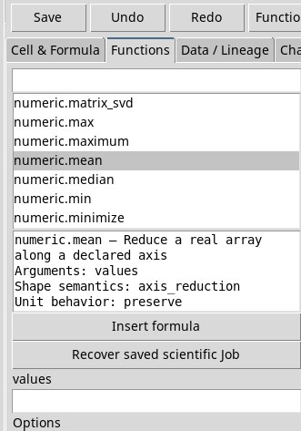
Set inputs, options, and model
Open an already registered Workspace. The guided editor creates a field for each exposed operand. You can enter cells, ranges, named columns or compatible literals. Text constants go in quotes. For example, when the provider wants a Dataset ID and a variable ID, use "worksheet_practice" and "voltage". The session field starts from @session when declared.
Leave optional trailing operands empty. To skip an intermediate operand, use empty() if the contract accepts it. For compound arguments the panel accepts the same typed constructors as formulas. For example, rf.calibration.one_port_apply accepts a record of coefficients in the known_standards argument. Some operations require more specific forms, such as two-dimensional matrices for points and rank-three tensors for a multiport RF sweep. Before the calculation, check that the source and the input can represent the required form. matrix has two dimensions. A single rectangular range of cells cannot directly represent a frequency × port × port sweep.
In Options takes chiave=valore pairs separated by spaces, with no spaces inside each pair. For example, third_shape=3 sets the third parameter of numeric.foundation.special.incomplete_beta. Leave it empty for the default values. When a model selector appears, choose the suitable declarative model and fill in its fields with the same key–value scheme. For example, the numeric.foundation.ode.solve panel shows linear_ode. Callback functions use the models allowed by the provider.
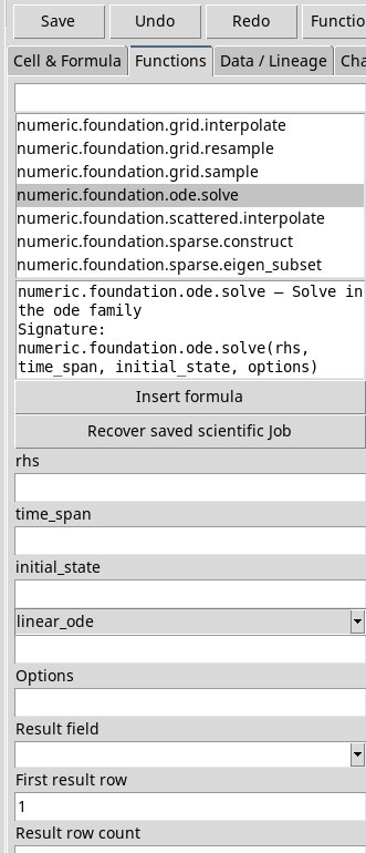
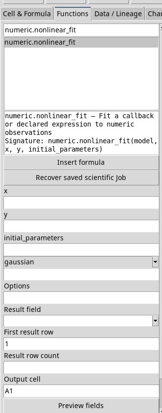
Identify a missing model operand
Compare the signature with the fields of the editor. In the tested version, numeric.polynomial_evaluate requires model and target_x. The panel only offers target_x and the provider rejects the Job, which receives only one argument. For a known polynomial, enter in a free cell =field(numeric.polynomial_evaluate(record("coefficients",vector(2,1)),vector(0,1,2)),"yq"). The result is 1, 3, 5, arranged in three rows from the active cell.
signal.filter.causal requires model, samples and an optional state. The editor shows samples and state. For the example without an initial state, write the record("numerator",vector(0.5,0.5),"denominator",1) model in the first field and, in the second, vector(1,3,5,7,9). After Preview fields apply value_real. The samples field occupies the position of the model, state that of the samples. This path offers no third box for the initial state.
You can also enter the cell call with =field(signal.filter.causal(record("numerator",vector(0.5,0.5),"denominator",1),vector(1,3,5,7,9)),"value_real"). With a zero initial state the values are 0.5, 2, 4, 6 and 8. The first value uses a zero previous input. From the second sample on, the filter averages the current sample and the previous one.
For the time response, signal.response.input requires a model, a grid and an input. The editor shows only two. For an in-cell example use =field(signal.response.input(record("kind","tf","numerator",1,"denominator",vector(1,1)),vector(0,0.25,0.5,0.75,1),vector(1,1,1,1,1)),"value_real"). The first-order system with a unit constant input returns samples of 1 − exp(−t), from 0 up to about 0.63212 at the last time.
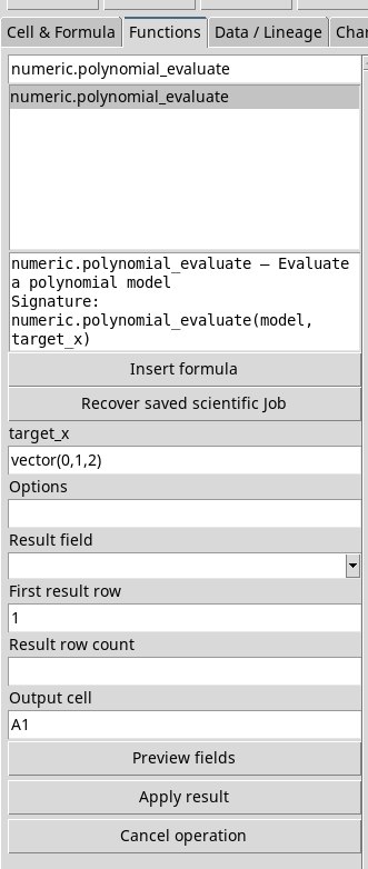
Start, cancel and read the Job status
Press Preview fields to submit the calculation. The status line shows the Job identity and the status reported by CORE Jobs. While the fields have not yet appeared, use Cancel operation to request a stop. The result is captured before being written. The Jobs bar of the main window lets you open the details and logs of the process, even when the status in Worksheet shows only a failure.
If the Workbook is a lightweight draft with no identity, you will read Save the Worksheet before managed scientific operation submission. In the verified version you can import the pre-registered template. If you change source, sheet, operands, options or editor while the Job is running, check the status again. The system may refuse to adopt a result that no longer matches the inputs.
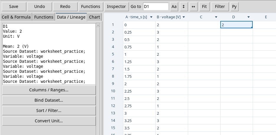
With many requests in the same Workbook, the registry may respond with Unsafe Registry source before creating the Job. In testing with 16 measurements, the refusal came at the eighteenth consecutive new request. The threshold varies with the state of the Workspace. Import another copy of the template with a different name, reopen it, select the original Dataset by ID and repeat the binding. The calculation of mean returned 2 V again and could be applied once more.
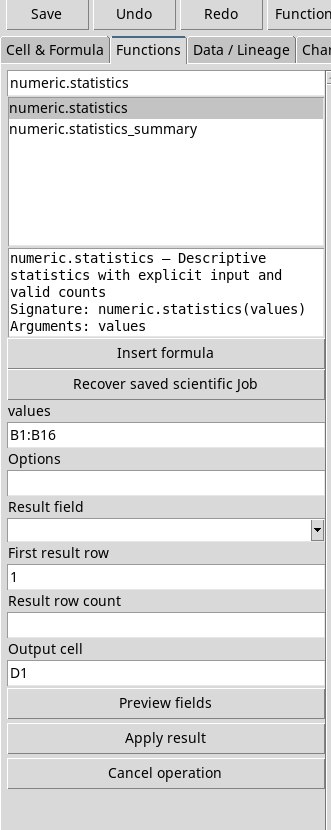
Apply a result field to empty cells
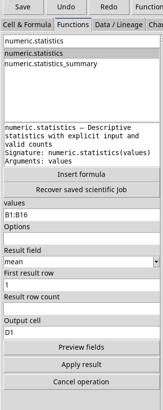
- After the capture, open Result field and choose one of the fields actually available. With a single field, the Viewer may already have selected it.
- Set Output cell to the start of a free area. First result row starts at 1, and an empty Result row count keeps the default behavior of the field. The row window applies to captured statistical results that support it. An FFT vector requires the window to be left empty, otherwise the Viewer refuses the request.
- Press Apply result. If there is no active Job yet, the button can start the capture. For a result with several fields, use the preview and the choice explicitly. Check the status, the cell value and Data / Lineage. Choosing the captured field and the destination does not require a new estimation.
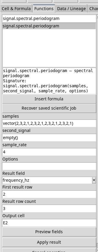
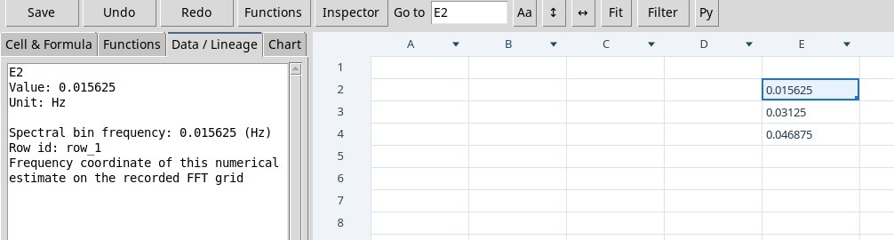
To try the window, choose signal.spectral.periodogram, put vector(2,3,2,1,2,3,2,1,2,3,2,1,2,3,2,1) in samples, empty() in second_signal and 4 in sample_rate. Start Preview, choose frequency_hz and set first row 2, count 3 and destination E2. With the default options the observed grid has a 0.015625 Hz step and the result occupies E2:E4. The n field, by contrast, is a scalar, and the same window exceeds its range.
Recover saved scientific Job tries to recover the last ticket of this Workbook. Workspace, Session, sources and inputs must match. If there is no saved ticket or its identity has changed, read the reason and launch a new calculation with verified inputs. Recovery was verified with the Workbook still open. The save defect prevents testing recovery after closing and reopening.
Lab with synthetic data
- Mean and variance
- With A1:B16 bound, choose
numeric.statisticsandB1:B16in values. After Preview choosemeanand apply it to D1. Result: 2 V. To compare it with the sample variance, use thevariance_samplefield in a new capture. Over a range of 16 measurements the variance is about 0.5333 V². - Discrete convolution
- Choose
signal.convolution.linear, x B1:B4 and kernel B1:B2. Leave the other fields empty and choosevalue_real. The five elements are 4, 12, 13, 8, 3. The convolution extends the sequence and uses the product of the amplitudes. Check the unit fields exposed by the provider separately. - Special function
numeric.foundation.special.erfwith value1returns about 0.842700793 invalue_real. Leave the operands not required by the case empty.- Magnetomotive force
- In
magnetics.circuit.mmfuses the quantities 5 and 2 as turns and current in the provider’s convention.value_realequals 10 and the operation also exposes aunitfield. - RF reflection coefficient
- For
rf.metric.reflectionuse network0.5. Thevalue_realfield returns 0.5 andvalue_imaginaryis the imaginary component. The coefficient is dimensionless.
Fit lab with a canonical Dataset
Import the models Dataset from the Dataset tab of the main window with Actions → Import Dataset ZIP…. Its eight x abscissas are positive. The six responses are synthetic and noise-free, each produced with the model of the same name. Open the exercise Workspace.
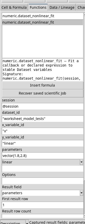
- In Functions choose
numeric.dataset_nonlinear_fit. Set session with@session, dataset_id with"worksheet_model_tests", x_variable_id with"x"and y_variable_id with"linear". The Job reads the canonical variables of the Session. - Choose
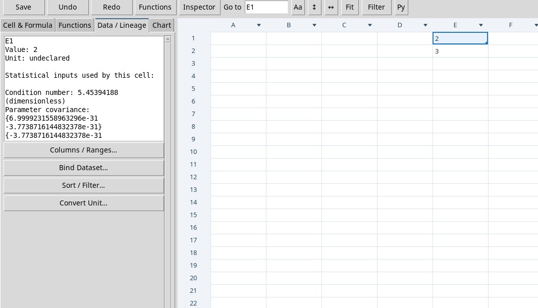
linearin the model selector. In parameters entervector(1.8,2.8). Use Preview fields, chooseparametersand apply it to E1, with E1:E2 free. You get intercept 2 and slope 3 within numerical rounding. - Select E1 in Data / Lineage. The sources are
xandlinear, there are 8 observations and 6 residual degrees of freedom. R² is 1 because the measurements reproduce the model relation exactly. With experimental data, also check the residuals, the numerical conditioning and the meaning of the parameter units. - Change y_variable_id, the model and the initial vector together to try the other curves. The catalog describes the choices and reports the tested configurations. Choose
predictedfor the fitted values orresidualsfor the residuals at the observed positions.
Lab with a geometric matrix and an RF record
Area of a triangle
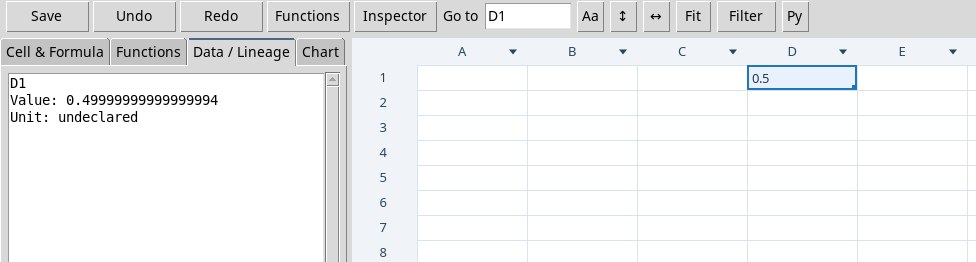
Choose numeric.foundation.geometry.triangle_area. Enter matrix(vector(0,0,0,1,0,0,0,1,0),1,9) in the first operand. Each row contains the coordinates of the three vertices, in this case (0, 0, 0), (1, 0, 0) and (0, 1, 0). Leave the other fields empty, run Preview fields and apply area to D5. The expected area is 0.5, i.e. half the product of the two unit legs. The literal has no declared unit. If you prepare the coordinates in meters, interpret the result consistently in square meters.
One-port calibration
- Choose
rf.calibration.one_port_solve. In the first two operands entervector(-0.88,0.02,0.92)andvector(-1,0,1). The three measurements correspond to the theoretical standards in the same order. Leave the third field empty. The estimate exposes directivity, tracking, source match and residual norm. Thedirectivity_realfield is about 0.02 in D3. - To correct a measured reflection of 0.47, choose
rf.calibration.one_port_applyand insert0.47in the first field, even though it has the shared label measured_standards. In the known_standards field, writerecord("directivity_real",0.02,"directivity_imaginary",0,"tracking_real",0.9,"tracking_imaginary",0,"source_match_real",0,"source_match_imaginary",0). Use Preview fields and applyvalue_realto D1. - The corrected value is 0.5 within numerical rounding. With real components and zero source match, it equals (0.47 − 0.02) / 0.9. Complex fields and source match must be kept when present in the calibration.
Test a mean with a t-test
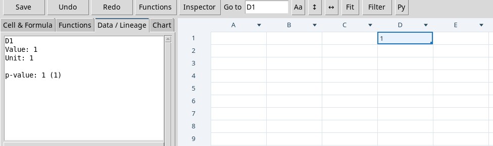
In Functions choose numeric.hypothesis_test. Put "one_sample_t" in method, vector(1,2,3,4,5,6) in first_values and empty() in second_values. In Options write mu0=3.5 alternative="two_sided". The explicit empty value keeps the operand required by the contract. After Preview fields apply p_value to D1. The result is 1 because the sample mean 3.5 coincides exactly with the reference and the t statistic is zero. Before using the test on measurements, check the independence of the observations and the adequacy of the t model.
Multiport RF sweep and tensor axes
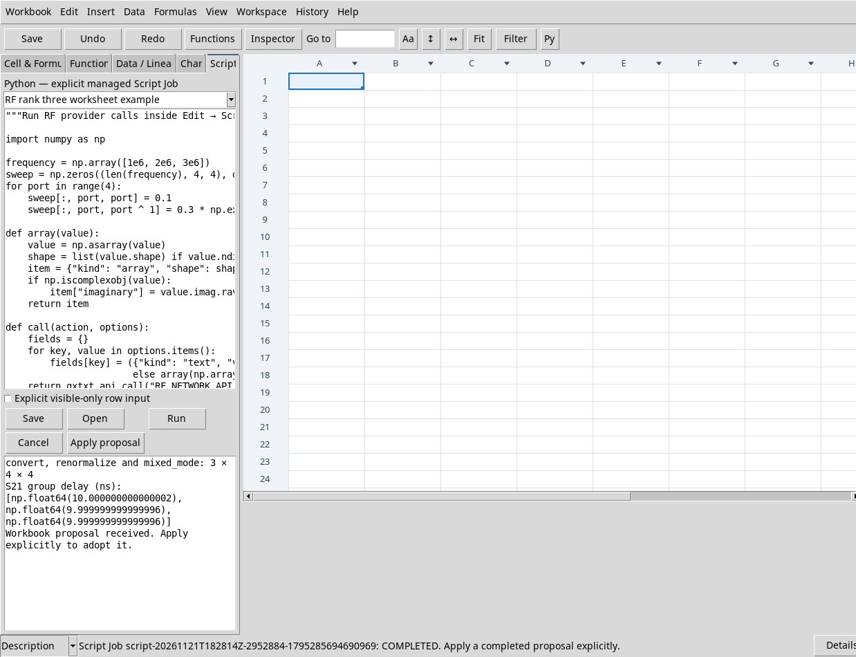
The multiport Dataset contains three increasing frequencies in Hz and, for each frequency, the real and imaginary parts of the S matrix. Each s_real and s_imag variable has shape 3 × 4 × 4. The first index identifies the frequency, the second the receiving port and the third the source port. The Worksheet table binding excludes rank-three variables. A 3 × 16 matrix entered in the panel was rejected by the four sweep operations.
Open a pre-recorded Workspace, then Edit → Scripts. Copy the contents of the RF Script (unzip the archive first), which regenerates the same synthetic values in memory. Press Run. The log verifies the S→Z conversion, renormalization from 50 Ω to 75 Ω and mixed-mode conversion for four ports. Also check that the group delay of S21 is 10 ns at the three samples. Apply proposal writes 10 in E1. For a single complex channel on a frequency grid there is also the rf.metric.group_delay function.
Keep the identity of a result for inference
- Dataset imports the Dataset of eight observations. It contains dimensionless X and Y, with an almost linear Y and a curvature term that the example can measure.
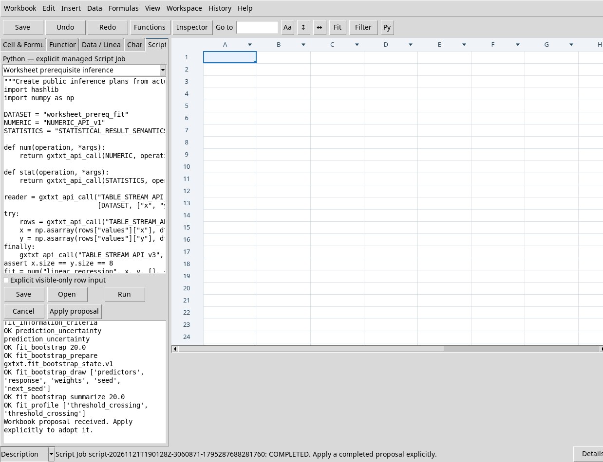
- Open Edit → Scripts in a pre-recorded Workspace. Paste the Inference script (unzip the archive first) and press Run. The script reads the observations from the Dataset, builds linear and quadratic fits and keeps, for both, the identity of the Dataset and of the ordered rows.
- Read the log. The nested F test compares the two fits on the same observations under the assumptions of independent Gaussian errors and estimated variance. The p-value in the example is about 0.000138. For the uncertainty of the parameters and of the mean response, the plan uses a nominal coverage of 95 %. The prediction requires exactly the fit parameters. A derived property, the information criteria and a 20-draw bootstrap with a reproducible seed are verified. Twenty draws are enough to test the tutorial path. The same script reuses the state and the log of the draws to verify the bootstrap summary. The likelihood profile uses a declarative fit with constrained refits. In the exercise it meets the threshold at both ends of the search. The profile coverage is approximate and conditional on the model and on the declared error law.
- Optionally apply the proposal to bring the slope coefficient into E1. The plans are prepared by the script through the public CORE contract and passed to the relevant calculations. The guided panel requires the corresponding public operands and their identity.
Typed grids, curve families and vector fields
For a rectilinear grid, prepare a list of two or three strictly increasing axes. The field is a matrix or tensor whose size along each index matches the length of the corresponding axis. sample and interpolate also require query coordinates as a matrix, one row per point. resample and compatible require a second list of axes. A matrix with all axes stacked was rejected.
Open Edit → Scripts, paste grid and field script (extract the ZIP first), and use Run. The planar field is f(x,y) = x + 2y on [0, 2]². Interpolating at the point (0.5, 1) gives 2.5. The integral is 12 and rises to 24 with a constant weight of 2. The cubic grid uses the same interval on each axis. The five curve-family functions use paired lists of abscissas and ordinates and a common comparison axis.
In the Magnetics actions, divergence and curl take an X × Y × Z × 3 tensor, with the last dimension for the components. The Laplacian requires a scalar XYZ field with at least three points per axis. The script checks that the divergence of the field (x, y, z) equals 3, that its curl is zero and that the Laplacian of x² + y² + z² equals 6. The log reports the individual outcomes.
Provide VTK volumes and meshes to guided operations
Download the VTK volume (unzip the archive first) and left mesh (unzip the archive first) and right mesh (unzip the archive first). Use the actual absolute paths, on a configuration with the VTK backend available. File input uses the @text:/percorso/al/file form. Use a writable destination folder for the outputs.
- volume_slice. Enter the volume in order,
vector(0,0,1.5)as the point andvector(0,0,1)as the normal. With Preview fields you access the points and scalars of the section at Z = 1.5. - mesh_smooth. Select
left.vtp. Options usesiterations=5 output_path="/percorso/smooth.vtp". The result includes path, hash and the counts of points and cells. - mesh_remesh. Use the same input mesh and
iterations=1 output_path="/percorso/remesh.vtp". Check the counts of the independent output. - mesh_boolean. Enter the two PolyData and
method="union" output_path="/percorso/union.vtp"files. The surfaces intersect so as to exercise the union. Read the path and the SHA-256 in the result.
Physical units and column-wise spectral output
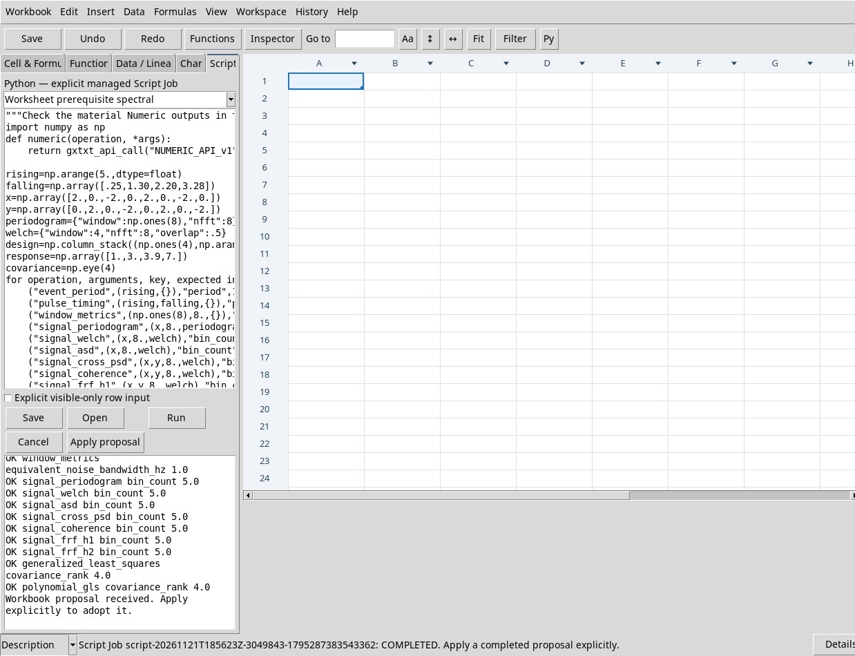
For the Numeric periodogram, use a window as long as the signal. For Welch, ASD, coherence, cross PSD and H1/H2 the test uses eight samples, window=4 nfft=8 overlap=0.5, a sampling frequency of 8 Hz and a second series of the same length where required. Once the window check was passed, the guided Job required an adapter with per-column facts instead of a scalar value per bin. With the spectral and GLS script (unzip the archive first) the provider returns five bins for all seven functions. The Signal · periodogram path returns applicable fields for frequencies and power. Use the physical parameters of the Signal contract when you choose that path.
For event_period and pulse_timing the test assigned s to both crossing columns. For window_metrics the coefficients are unity, with unit 1 and a sampling frequency of 8 Hz. The Numeric guided path still returned the refusal relating to the CORE contract. For a sampled signal, see Signal · period from events and check the threshold, the time unit and the sample range. In the script log, the period is 1 s, the mean duration is 0.2575 s and the equivalent noise bandwidth of the window is 1 Hz.
The same script tests GLS regression with an absolute identity covariance, then with a rank-four one. For general covariances, rows and columns must refer to the same order of observations, and the unit must be compatible with the square of the response unit. In the guided editor, adding covariance_unit produces Unknown GLS option; leaving it out produces the refusal for the missing key.
Pass recipes and models while keeping the public state
A prediction requires the model declaration and the query coordinates. A model obtained from a fit can also contain the observed domain, units, parameter identities and scales. In Cell & Formula you can build a simple model with a record. For a model produced by the provider, keep the complete object, especially when a function requires the state of the saved model or a branch with a defined domain.
Open Edit → Scripts and paste the model script (unzip the archive first). The log runs through recipe, fit, evaluation, residuals and any state. The tutorial surface z = 3 + 2 x + y gives 3 at the origin and zero residuals at the exact points. In the rational model the denominator is normalized with constant term 1 and is checked over the domain [0, 4]. The complex case uses frequency in Hz, impedance in Ω and the absolute covariance of the two components. The implicit case declares the response branch with two bounds and a residual scale in V. In the regional model, the windows [0, 4] and [6, 10] exclude the intermediate samples. The composite model makes five distinct parameters available for a Lorentzian peak and a linear baseline.
Check the covariance of a digitization
Open Edit → Scripts and use the two-point digitization script (unzip the archive first). The physical coordinates are in mm. The recipe includes a local Jacobian from pixels to coordinates and a calibration Jacobian for two common offsets. The first calculation uses independent physical standard uncertainties of 0.02 and 0.03 mm. In the second, each point has an independent localization with a rectangular distribution and the same calibration. A width of one pixel corresponds to a standard deviation of 1/√12 pixel.
To compute the covariance, pass the complete result of digitization_uncertainty to digitization_covariance. In X the covariance between the two points is zero in the independent case and 0.0004 mm² in the shared case. The x and y choices produce 2 × 2 matrices; xy produces a 4 × 4 matrix in the order X1, Y1, X2, Y2. The log verifies that the identity of the result stays the same in the three calculations. The complete matrix is limited to 512 points.