2D21 Thyratron: From GE Datasheet Curves to a Level-1 Compact Model

Introduction

The 2D21 is a small gas thyratron designed for control and switching applications. Historical datasheets do not describe its behavior with a single equation, but through several families of characteristic curves.

In this first study I focus on only one of these families: control-grid current during anode conduction. The quantity I want to describe is therefore:

\[ I_g = F(V_g,I_a) \]

where:

• \(V_g\) is the control-grid voltage;
• \(I_g\) is the control-grid current;
• \(I_a\) is the anode current, which identifies the different curves in the family.

Thyratron grid behavior is of course not a new problem. Grid current, critical control-grid potential, firing, and the behavior of a grid immersed in plasma already appear in the early work on these devices that I consulted.

In 1931 W. B. Nottingham published measurements of grid current, critical grid potential, and other characteristics of small thyratrons [Nottingham, 1931].

In 1954 Mullard published Thyratrons for Industrial Control, a treatment devoted to thyratrons for industrial applications that also includes characteristics of ionic grid current during conduction [Mullard, 1954].

A particularly useful physical treatment is H. H. Wittenberg’s chapter Gas Tube Design, included in the 1962 volume Electron Tube Design [Wittenberg, 1962].

Wittenberg describes the grid, during thyratron conduction, as a probe immersed in the plasma. The current collected by the grid results from contributions from ions and electrons and depends on discharge conditions. This provides an important physical basis for understanding why grid current depends not only on the voltage applied to the grid, but also on anode current and, more generally, on the state of the plasma inside the tube.

Document note: the copy of Electron Tube Design that I used comes from Wikimedia Commons, where the work is marked as Public Domain. The PDF is also hosted on Giux-Lab for easier consultation. For details on its public-domain status and any territorial limitations, please refer to the source page.

There is also a direct precedent for SPICE simulation of the 2D21: the macromodel developed by Zabb Csaba. The author states that it is applicable to PL21, 2D21, and 21TE31 thyratrons and publishes it in his SPICE model collection [SPICE Models – Zabb Csaba].

Zabb also provides a short document dedicated to the model [Thyratron Macro Model – PDF]. The document shows several practical applications: a relaxation oscillator, including a comparison between simulation and experimental measurements, and a timebase circuit of the type used in early oscilloscopes.

Zabb’s macromodel is therefore an important precedent, and it would be incorrect to present this work as the first mathematical model or the first SPICE model applicable to the 2D21. The problem I want to address here, however, is different.

In the sources I examined, I did not find a quantitative compact model of the 2D21 derived directly from the complete family of manufacturer characteristics:

\[ I_g = F(V_g,I_a) \]

with a documented procedure for parameter extraction, uncertainty analysis, and quantitative comparison with the curves used to build the model.

For this reason I started from the characteristics published by General Electric. I digitized the curves several times using independent calibrations and then combined them to obtain a consensus curve and an estimate of the dispersion introduced by the digitization process.

The datasheet contains the families corresponding to:

\[ I_a = 5,\ 25,\ 50,\ 100,\ 150,\ 200,\ 300\ \mathrm{mA} \]

I identified the main model structure primarily using the families from \(25\) to \(200\ \mathrm{mA}\). I also used the \(300\ \mathrm{mA}\) curve in robustness checks, while I kept the \(5\ \mathrm{mA}\) curve separate as a check for possible different behavior at low current.

The goal was not simply to find an independent equation for each curve. A set of separate fits could have reproduced the original graph well, but would have provided little information about the common structure of the entire family.

I therefore looked for a representation in which the different curves could be described by common mathematical functions and a limited number of parameters specific to each family.

The result of this work is the 2D21 Level-1 v0.1 model.

Its scope is deliberately limited. The model describes only:

\[ I_g = F(V_g,I_a) \]

during anode conduction.

It does not yet describe:

• thyratron firing;
• discharge extinction;
• deionization and recovery;
• the effect of the second grid \(G_2\);
• the complete time-domain dynamics;
• the complete SPICE behavior of the device.

In this article I will show, step by step, which curves I started from, how I digitized them, how I transformed the data, and how I arrived at the final mathematical structure. I will also show where the model reproduces the original characteristics well, where differences remain, and what its limitations are.

I now consider the mathematical structure of version 0.1 frozen. I will therefore not add further parameters merely to improve the fit to the same General Electric curves.

In a separate study I will test the same structure against characteristics published by other manufacturers, in order to establish how far the model can be generalized. In parallel, for the original Flash-Matic objective, I can implement this static law as one of the sub-blocks of a future 2D21 SPICE macromodel, without confusing circuit implementation with validation on other devices.

The proposed model

Before describing how I digitized the curves, how I chose the parameters, and why I arrived at this mathematical form, I prefer to show the result first.

The 2D21 Level-1 v0.1 model describes the control-grid current during anode conduction:

\[ I_g = F(V_g,I_a) \]

The first step is to normalize grid current with respect to anode current:

\[ Y=\frac{I_g}{I_a} \]

The characteristic is then divided into two regions around the voltage \(V_0\), defined as the point at which grid current changes sign:

\[ I_g(V_0)=0 \]

The complete normalized model is:

\[ Y = \begin{cases} G_-(X_-;Q_A,U_{20}), & V_g \le V_0 \\[2mm] G_+(X_+;K), & V_g > V_0 \end{cases} \]

with:

\[ X_-=\frac{V_g-V_0}{S_-} \]

and:

\[ X_+=\frac{V_g-V_0}{S_+} \]

Positive branch

For \(V_g > V_0\), the model uses:

\[ G_+(X;K) = 0.005 \frac{\exp(KX)-1} {\exp(K)-1} \]

For the 2D21, the identified value is:

\[ K \approx 0.551 \]

Negative branch

For \(V_g \le V_0\), the model uses:

\[ G_-(X;Q_A,U_{20}) = -Q_A+ \sum_{j=1}^{3}A_j\exp(\lambda_jX) \]

with three exponential coefficients characterized by the constants:

\[ \lambda_1=0.060 \]

\[ \lambda_2=0.240 \]

\[ \lambda_3=0.960 \]

that is, in the ratio:

\[ 1:4:16 \]

The coefficients \(A_1\), \(A_2\), and \(A_3\) are not free model parameters. I calculate them from two geometric parameters of the individual family, \(Q_A\) and \(U_{20}\), by imposing three conditions:

\[ G_-(0)=0 \]

\[ G_-(-1)=-0.01 \]

\[ G_-(-U_{20})=-0.020 \]

I finally recover the actual grid current from the normalized form:

\[ I_g=I_a\,Y \]

Parameters of an individual family

For each anode-current value, the model requires five quantities:

\[ V_0,\qquad S_-,\qquad S_+,\qquad Q_A,\qquad U_{20} \]

These quantities determine the position of the curve, its voltage-axis scales, and the shape of the negative-grid-current region.

In version 0.1 I determine these parameters separately for each anode-current family. The notation \(I_g=F(V_g,I_a)\) therefore identifies the family through \(I_a\), but does not yet imply that the model can automatically interpolate the parameters at an arbitrary anode-current value.

The mathematical structure instead remains common to the different families. This is the central point of the model: rather than using an independent equation for each curve, I use a common structure capable of representing them all by changing only a small set of parameters.

What the model describes — and what it does not

The two branches are continuous at \(V_0\):

\[ G_-(0)=G_+(0)=0 \]

The model is therefore continuous in current, but I do not impose equal slopes for the two branches at the crossing point. In mathematical terms the model is C0, but not C1. As I will show later, this choice is not arbitrary: forcing derivative continuity produces a much worse agreement with the digitized curves.

It is also important to remember that this equation does not yet represent the complete behavior of the thyratron. It describes only the family:

\[ I_g(V_g,I_a) \]

during anode conduction. Triggering, extinction, recovery, the second grid, and dynamic behavior must be addressed separately.

In the following sections I will show where these equations come from, what the individual parameters represent, and why I preferred this structure to apparently simpler alternatives.

This model therefore represents the first necessary step toward the final objective: obtaining a 2D21 model usable in SPICE and, if the structure proves sufficiently general, extendable to other thyratrons of the same broad class.

The datasheet and the starting graph

The starting point for the model is the original General Electric 2D21 datasheet. I make available here the copy I used for this work: [General Electric 2D21 – datasheet PDF].

Among the various characteristics reported in the document, the one used in this first phase is the Average Characteristics During Anode Conduction graph. It shows control-grid current \(I_g\) as a function of grid voltage \(V_g\), for several values of anode current \(I_a\).

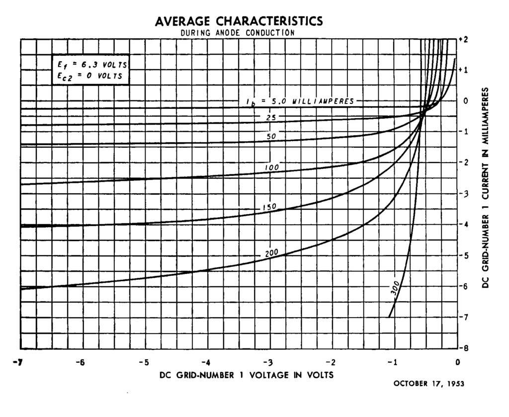
Because the datasheet provides these characteristics only in graphical form, my first step was to turn them into numerical data. To do this I used Curve Digitizer, the software I developed to calibrate graph axes and digitize curves.

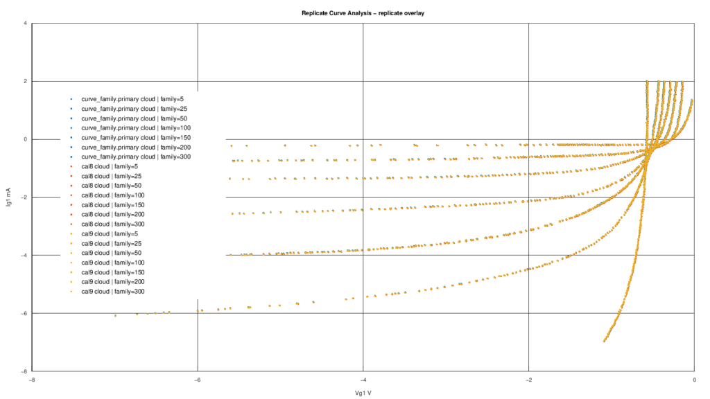
I did not perform the digitization only once. I carried out multiple independent acquisitions and calibrations of the same graph so that I could later compare the results and estimate how much the image-reading process affects the resulting data.

In the next step I will show what data I obtained from these digitizations and how I combined them before using them to build the model.

From digitizations to the consensus dataset

A single digitization of a graph cannot be treated as an exact datum. Point positions depend on axis calibration, image resolution, and the manual selection of points along the curves.

For this reason I did not use a single acquisition directly. I digitized the characteristics several times using independent calibrations and then compared the results.

For this phase I used my analysis framework, GX-TXT Pipeline, developed in Tcl/Tk. The program is built around a defined API that allows independent analysis modules to be added without modifying the software core. I plan to publish the framework shortly.

The module I used in this case is:

curve.replicate_analysis

Its task is not to fit the physical model, but to compare replicated digitizations, construct a consensus curve, and estimate the uncertainty associated with the digitization process.

Replicated digitizations

For each anode-current value I compared three independent sources of the same curve. With seven anode-current families, this corresponds to 21 sets of points.

The files do not contain an explicit identifier for each individual repetition. I therefore treated the data as unlabeled point clouds: I do not use CSV row order and I do not interpret it as experimental information.

I also did not infer the number of independent measurements from the number of digitized points. A curve with many points does not automatically represent a larger number of independent experiments; it simply indicates a denser digitization.

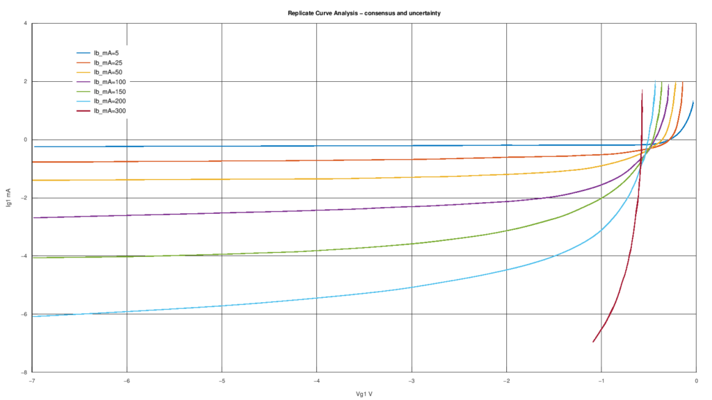
Building the consensus curve

For each source and each family, the module constructs a local representation of the curve using local linear regression. I compare the sources only over the voltage interval common to the different digitizations, without extrapolating beyond the domain actually covered by the data.

From these representations I obtain a mean consensus curve, subsequently sampled on a uniform grid of about 300 points per family.

These 300 points must not be interpreted as 300 independent measurements. They are simply a sufficiently dense numerical representation of the consensus curve, useful for fitting and residual analysis.

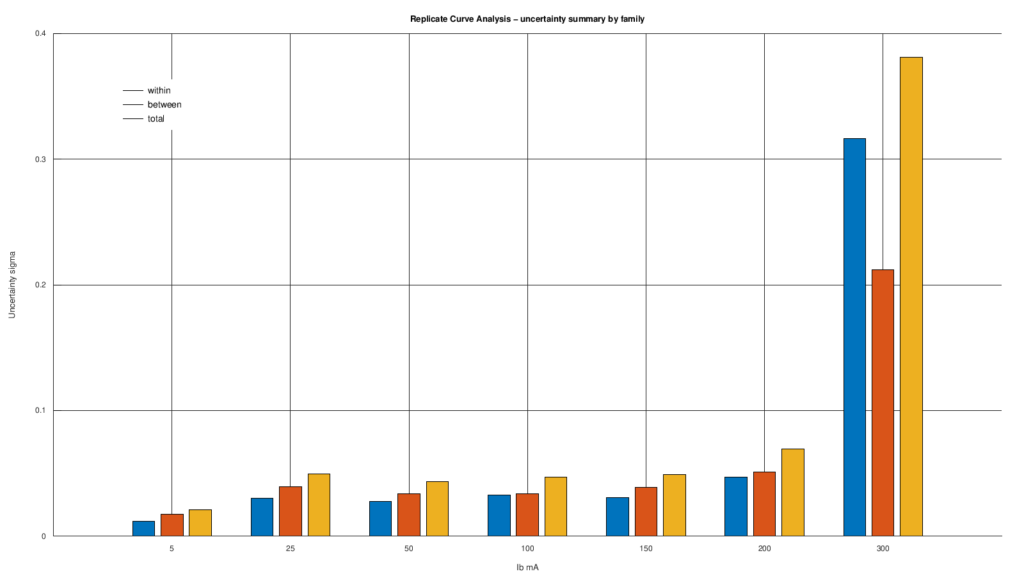
Estimating uncertainty

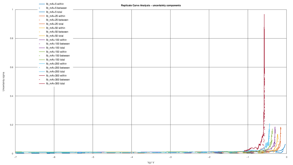
I separated the uncertainty into two contributions.

The first, which I denote as:

\[ \sigma_{\mathrm{within}} \]

describes the local dispersion of points around the reconstructed curve within the individual sources.

The second:

\[ \sigma_{\mathrm{between}} \]

measures how much the curves obtained from the different digitizations and calibrations differ from one another.

I combined the two contributions as:

\[ \sigma_{\mathrm{total}} = \sqrt{ \sigma_{\mathrm{within}}^2 + \sigma_{\mathrm{between}}^2 } \]

This is the uncertainty I use later to evaluate how large the deviations between model and data are relative to the dispersion introduced by digitization.

For fitting and residual evaluation I did not use the standard error of the mean as the primary uncertainty. The objective is to represent the dispersion of the digitization and calibration process, not merely the precision with which the mean curve is estimated. For this reason, in the following checks I use \(\sigma_{\mathrm{total}}\), which preserves the scale of the variability observed among the digitizations.

A special case: the 300 mA curve

The analysis immediately shows that the \(300\ \mathrm{mA}\) family is much more uncertain than the others. Its useful voltage interval is also much shorter because the original curve covers only the region near the transition.

This difference becomes important later: the \(300\ \mathrm{mA}\) curve remains useful for testing the model structure, but it does not allow all parameters to be determined with the same reliability as the families between \(25\) and \(200\ \mathrm{mA}\).

1 / 4

Open the full gallery page Download gallery ZIP (HTML + hi-res images)

Data reproducibility

At this point the starting data are already independently reproducible: I have identified the original datasheet used and the Curve Digitizer software with which I numerically extracted the curves from the graph.

Anyone wishing to repeat the work can therefore start from the same image and perform an independent digitization of the characteristics.

For the next phase—the automatic construction of the consensus curve and its uncertainty estimate—I used the curve.replicate_analysis module of my GX-TXT Pipeline framework. The framework has not yet been published, but I intend to make it available shortly together with the modules used in this analysis.

Until then, I describe here the procedure I used and the quantities I calculated, so that data obtained directly from digitization can be clearly distinguished from the subsequent statistical processing.

From consensus curves to the search for a common shape

Once the consensus curves have been obtained, the next problem is to determine whether the different families have something in common or whether they must be described as completely independent curves.

The first transformation I tried was dividing grid current by the anode current of the corresponding family: \[ Y=\frac{I_g}{I_a} \]

This makes \(Y\) dimensionless and allows curves obtained at very different anode currents to be compared directly.

The purpose of the transformations that follow is not to alter the data in order to force the curves to overlap artificially. Rather, the idea is to separate purely geometric differences—amplitude, position, and scale—from differences that represent a real change in the shape of the characteristic.

A simple example may help. Two curves may have exactly the same shape, but one may be taller than the other, shifted horizontally, or wider. In the original coordinate system they would appear different; after properly correcting scale and position they might instead overlap.

If this happens, it means there is no need to construct a completely different formula for every anode-current value. The different characteristics can be interpreted as transformed versions of the same underlying mathematical structure.

The procedure I followed on the 2D21 is therefore progressive. Each step attempts to remove one source of difference between the curves and then examines what remains.

The first step is the vertical normalization already introduced: \[ Y=\frac{I_g}{I_a}. \]

I then identify, for each family, the voltage \(V_0\) at which grid current changes sign: \[ I_g(V_0)=0. \]

Subtracting \(V_0\) from grid voltage brings all curves to the same reference point: \[ \Delta V = V_g-V_0. \]

This allows me to test whether the observed differences are due only to a horizontal shift. As I will show, however, zero alignment is not sufficient: the curves also have different horizontal scales.

For this reason I treat the two sides of the characteristic separately. On the branch where grid current is negative I introduce a scale \(S_-\), while on the positive branch I use a scale \(S_+\): \[ X_-=\frac{V_g-V_0}{S_-} \]

and \[ X_+=\frac{V_g-V_0}{S_+}. \]

The quantities \(X_-\) and \(X_+\) are not voltages: they are dimensionless coordinates. They are used to compare curve shapes after removing both their displacement and their different extent along the voltage axis.

At this point the question becomes very concrete:

once differences in amplitude, position, and scale have been removed, do the different 2D21 families become manifestations of the same fundamental curve?

The answer is not the same on the two branches of the characteristic. The positive branch behaves very nearly like a single common normalized curve, whereas small but systematic shape differences remain on the negative branch and require additional parameters to describe them.

The following graphs show this process one step at a time. For each one I will indicate the mathematical transformation applied, its geometric meaning, and above all what comparison among the different families allows me to infer.

1. First normalization: \(Y=I_g/I_a\)

The first step is to compare the different families after removing the most obvious difference: each curve was obtained at a different anode current \(I_a\).

For each point on the characteristic I therefore divided grid current \(I_g\) by the anode current of the corresponding family: \[ Y=\frac{I_g}{I_a}. \]

The result is shown in the following graph. The horizontal axis still contains the original grid voltage \(V_g\), while the vertical axis no longer shows grid current in milliamperes but the dimensionless ratio \(I_g/I_a\).

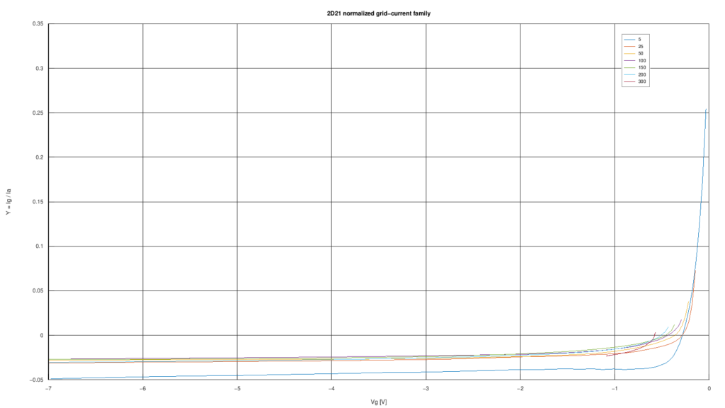
This transformation can be interpreted simply. If grid current varied in direct proportion to anode current—that is, if doubling \(I_a\) also doubled \(I_g\) while leaving the shape of the characteristic unchanged—then dividing by \(I_a\) should make the different families coincide.

The graph shows that this happens only partially.

On the negative-grid-current branch, the families from 25 to 300 mA are much closer to one another than they would appear when considering \(I_g\) directly. A substantial part of the variation of grid current with anode current can therefore be absorbed by the simple normalization \(I_g/I_a\).

This is already a useful result: it suggests that \(I_a\) provides a natural scale for comparing the different characteristics. It does not mean, however, that grid current is simply proportional to anode current. If that were the case, all curves would overlap after normalization, which clearly does not happen.

I also observe that the 5 mA family behaves noticeably differently. In particular, it reaches larger negative values of \(I_g/I_a\) in absolute magnitude and, on the positive branch, departs markedly from the families obtained at higher anode currents. For this reason, in the analyses that follow I treat the 5 mA curve with particular care as a possible low-current operating regime.

There is another immediately visible difference. The various curves do not cross \(Y=0\) at the same grid voltage.

In other words, even after removing much of the vertical difference, the characteristics remain horizontally shifted relative to one another. This suggests that the next step should be to identify, for each family, the voltage \(V_0\) at which grid current changes sign: \[ I_g(V_0)=0. \]

In the next graph I therefore show what happens when I shift each characteristic using its own \(V_0\) value.

2. Aligning the curves at the zero crossing: \(\Delta V = V_g – V_0\)

After the vertical normalization \(Y=I_g/I_a\), the different families are easier to compare, but an obvious difference remains: the point where grid current changes sign does not occur at the same voltage for all curves.

For each family I therefore identify the voltage \(V_0\) such that: \[ I_g(V_0)=0. \]

I then introduce a new horizontal coordinate: \[ \Delta V = V_g – V_0. \]

The transformation is simply a translation of the voltage axis. I shift each curve horizontally by its own \(V_0\) value, so that the point at which grid current becomes zero always falls at: \[ \Delta V = 0. \]

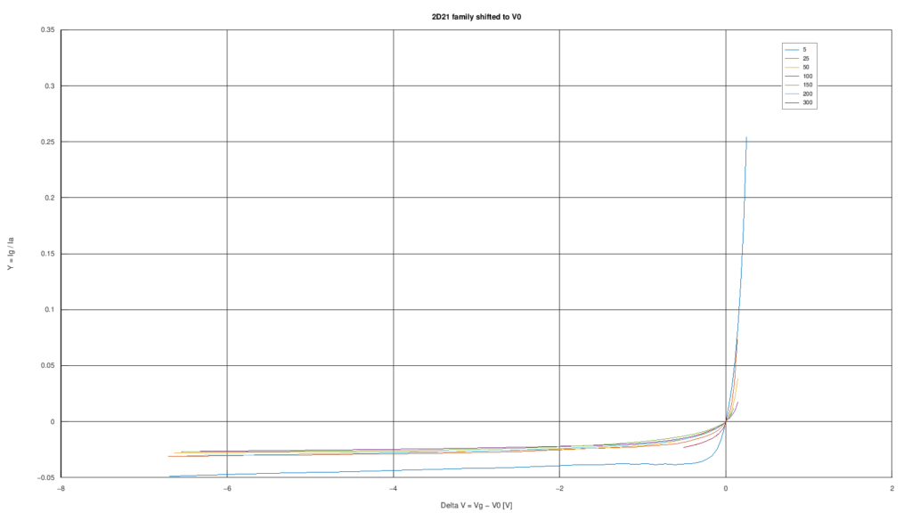
The geometric meaning of the graph is immediate: all families now pass through the same point \((\Delta V,Y)=(0,0)\).

This transformation allows me to test a very simple hypothesis: the curves might have the same shape and differ only by a shift along the grid-voltage axis.

If that were true, after subtracting \(V_0\) the different characteristics should overlap almost completely.

The graph shows that this is not the case.

Zero alignment correctly removes the positional difference, but the curves retain different horizontal extents. Some reach the same change in \(Y\) within only a few tenths of a volt, whereas others require a wider voltage variation.

This means that \(V_0\) describes only one aspect of the family: it identifies where net grid current changes sign, but by itself it does not determine how rapidly the characteristic evolves as one moves away from that point.

I also observe that the two sides of zero do not appear to behave in the same way. The branch with \(Y<0\) and the one with \(Y>0\) show different scales and curvatures as anode current changes.

This suggests that a single horizontal scale should not be used for the entire characteristic, and that the two branches should instead be treated separately.

For the negative branch I therefore introduce a characteristic scale \(S_-\), while for the positive branch I use a distinct scale \(S_+\).

The next step is to test whether, after normalizing this different horizontal scale as well, the families can be reduced to a common shape.

3. Normalizing the negative branch: \(X_-=(V_g-V_0)/S_-\)

After normalizing grid current to anode current and aligning all curves at their own zero crossing \(V_0\), one evident difference remains: the negative branch does not have the same horizontal extent for all families.

To compare this part of the characteristic more effectively, I therefore introduce a specific voltage scale, denoted \(S_-\), and a new dimensionless coordinate: \[ X_-=\frac{V_g-V_0}{S_-}. \]

I do not choose \(S_-\) arbitrarily. For each family I define it so that the point where normalized current is \(-0.01\) always falls at the same position: \[ Y=-0.01 \qquad\Longrightarrow\qquad X_-=-1. \]

In other words, after having already made all curves pass through \((0,0)\), with this transformation I also fix a second common point. This removes much of the difference in horizontal scale among the characteristics.

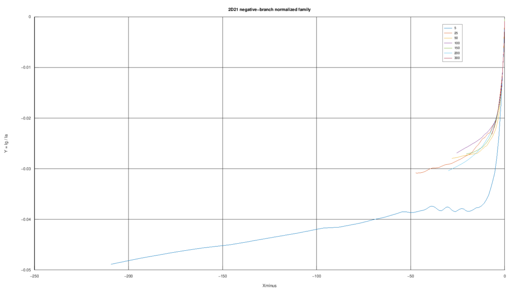
It is important to remember that \(X_-\) is no longer a voltage measured in volts. It is a dimensionless coordinate: it indicates how far I have moved from \(V_0\) relative to the characteristic scale \(S_-\) of the individual family.

For this reason some curves, especially the 5 mA curve, reach numerically very large values of \(X_-\). This does not mean that hundreds of volts were applied; it simply means that, for that family, \(S_-\) is very small compared with the voltage interval covered by the curve.

At this point I can test a stronger hypothesis than the one considered in the previous graph. After removing:

• the vertical scale through \(I_g/I_a\);
• the horizontal shift through \(V_0\);
• the different horizontal scale through \(S_-\);

the negative-branch curves should overlap if they were simply rescaled versions of the same function.

The graph shows a much better result, but the overlap is not complete.

The different families clearly follow a common trend, but systematic differences remain both in the depth reached by the negative branch and in the way the curve moves from the region near zero toward the more distant region.

This is an important result. It means that the shape of the negative branch cannot be described by a single universal function of \(X_-\) with no additional parameter: \[ Y \neq G_-(X_-) \]

with the accuracy required by the data.

The subsequent analysis showed that the residual differences can be described compactly by introducing only two geometric quantities.

The first, denoted \(Q_A\), describes the depth toward which the negative branch tends: \[ Q_A=-\lim_{X_-\rightarrow-\infty}G_-(X_-). \]

Intuitively, \(Q_A\) therefore represents the normalized negative plateau level.

The second quantity, denoted \(U_{20}\), instead describes how rapidly the curve moves toward that plateau. I define it through the point at which: \[ G_-(-U_{20})=-0.020. \]

\(U_{20}\) can therefore be read directly as a measure of the curve’s horizontal shape: it indicates how far one must move away from zero, in the normalized coordinate \(X_-\), to reach \(Y=-0.02\).

The result is therefore not a perfect negative master curve, but something that is still very useful: the different families can be reduced to the same mathematical structure using a scale \(S_-\) and only two geometric shape parameters, \(Q_A\) and \(U_{20}\).

On the positive branch, as I will show in the next graph, the result is even simpler: after normalizing the horizontal scale, the main families collapse much more completely.

4. Normalizing the positive branch: \(X_+=(V_g-V_0)/S_+\)

On the positive branch I apply the same idea used for the negative one: after normalizing the current and aligning all curves at their own \(V_0\), I introduce a specific horizontal scale, denoted \(S_+\).

The new dimensionless coordinate is: \[ X_+=\frac{V_g-V_0}{S_+}. \]

Here too I define \(S_+\) through a common reference point. For each family I choose the scale so that: \[ Y=+0.005 \qquad\Longrightarrow\qquad X_+=1. \]

In this way I compare all positive curves after removing three main differences:

• the different vertical scale, through \(Y=I_g/I_a\);
• the different zero crossing, through \(V_0\);
• the different horizontal scale, through \(S_+\).

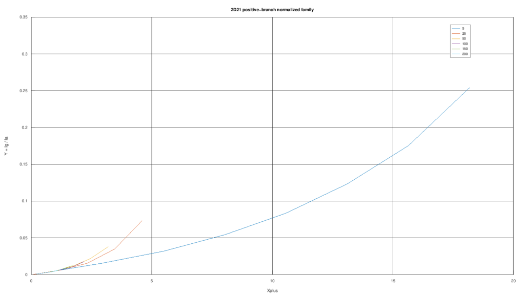
\(X_+\) is also a dimensionless coordinate rather than a voltage measured in volts. The value \(X_+=1\) simply identifies the point chosen as the reference for positive-branch normalization.

The graph immediately shows one peculiarity: the 5 mA family occupies a much larger region than the others, reaching substantially higher values of both \(X_+\) and \(Y\).

This behavior visually compresses the 25–200 mA families into the lower-left portion of the graph. It is therefore important not to interpret the overall scale of the image as evidence of poor overlap among these curves.

When the main families are examined separately, the result is in fact much stronger than on the negative branch: once the transformations have been applied, the 25–200 mA curves have very similar shapes.

This means that, on the positive branch, much of the dependence on anode current can be described simply by changing \(V_0\) and \(S_+\), without introducing additional family-specific shape parameters.

The common structure I identified can be described by: \[ G_+(X_+;K) = 0.005\, \frac{e^{KX_+}-1}{e^K-1}, \]

where \(K\) determines the curvature of the function.

For the 2D21, global analysis of the main families gives: \[ K \approx 0.551. \]

The significance of this result is particularly important: for the 25–200 mA families I did not need to assign a different \(K\) value to each curve. A single mathematical shape, combined with the respective \(V_0\) and \(S_+\) values, describes the whole group well.

In other words, the positive branch behaves very nearly like a true master curve: curves obtained at different anode currents can be brought to the same shape through simple position and scale transformations.

The 5 mA family instead continues to show different behavior. For this reason I did not use it to determine the main model structure and kept it as a possible low-current operating regime.

The 300 mA family is also absent from the graph. The reason follows directly from the definition of \(S_+\): in the available data this curve does not reach \(Y=+0.005\), so the point needed to determine \(S_+\) geometrically is not present.

I can subsequently estimate \(S_+\) for the 300 mA family using the model, but I do not treat that value as a quantity obtained directly from the normalization point.

Comparison of the two branches therefore leads to an interesting result. On the negative branch two additional geometric variations remain, described by \(Q_A\) and \(U_{20}\); on the positive branch, by contrast, the main families can be reduced to a single form with one common curvature parameter \(K\).

5. What I learned from the transformations

The four previous steps finally make it possible to view the 2D21 characteristic family differently from the original datasheet curves.

The first result is that the different curves do not appear to be completely independent characteristics. A substantial part of their differences can be removed through simple scale and position transformations.

The normalization

\[ Y=\frac{I_g}{I_a} \]

shows that anode current \(I_a\) provides a useful vertical scale: the main families become much more comparable when I express grid current as a fraction of anode current.

The subsequent alignment through \(V_0\) removes the difference in the position of the point where grid current changes sign:

\[ I_g(V_0)=0. \]

Even after this transformation, however, the curves retain different horizontal extents. This led me to introduce two separate scales, \(S_-\) and \(S_+\), for the negative and positive branches, respectively.

It is at this point that the two sides of the characteristic begin to show different behavior.

On the positive branch, after applying the transformations

\[ Y=\frac{I_g}{I_a}, \qquad X_+=\frac{V_g-V_0}{S_+}, \]

the main families from 25 to 200 mA can be reduced, with good accuracy, to the same mathematical shape. In this case most of the anode-current dependence therefore appears to be contained in \(V_0\) and \(S_+\), while the residual curve shape remains essentially common.

The negative branch is slightly more complex. The transformation

\[ X_-=\frac{V_g-V_0}{S_-} \]

also brings these curves much closer to one another, but does not produce complete overlap. Systematic differences remain in the depth of the negative branch and in the way the curve approaches that region.

The analysis showed that these differences can be described by only two additional geometric quantities: \(Q_A\), which characterizes the normalized negative plateau level, and \(U_{20}\), which describes the position of the curve at \(Y=-0.02\).

The overall result is therefore simpler than it may appear when looking directly at the original characteristics.

The different families do not necessarily require a completely independent formula for every value of \(I_a\). Instead they can be described through a common structure in which only a relatively small number of geometric parameters change.

Conceptually, the result can be summarized as follows:

\[ \text{original curve} \;\longrightarrow\; \text{vertical scale} \;\longrightarrow\; \text{common zero} \;\longrightarrow\; \text{horizontal scale} \;\longrightarrow\; \text{residual shape}. \]

The most important part of this procedure is therefore not that I found a transformation capable of making the curves look more similar, but that I identified which characteristics genuinely change from one family to another and which can instead be reduced to a common mathematical structure.

At this point I can use these results to construct a compact model of 2D21 grid current. In the next step I combine the geometric transformations just introduced into a single mathematical formulation and test how accurately it reproduces the characteristics from which I derived it.

The compact model of 2D21 grid current

The transformations discussed in the previous section progressively separated differences in scale and position from genuine differences in the shape of the characteristics.

At this point the results can be collected into a single mathematical model of 2D21 grid current.

The basic idea is fairly simple: instead of building an independent formula for each anode-current value, I use the same mathematical structure and let a small number of geometric parameters describe the differences among the various families.

I first express grid current in normalized form: \[ Y=\frac{I_g}{I_a}. \]

The point \(V_0\) naturally divides the characteristic into two regions:

• for \(V_g \leq V_0\), grid current is negative;
• for \(V_g > V_0\), grid current is positive.

The two branches use different normalized coordinates: \[ X_-=\frac{V_g-V_0}{S_-} \]

for the negative branch, and \[ X_+=\frac{V_g-V_0}{S_+} \]

for the positive branch.

The complete model can therefore be written compactly as: \[ I_g(V_g,I_a)= I_a \begin{cases} G_-\!\left(X_-;Q_A,U_{20}\right), & V_g\leq V_0 \\[3mm] G_+\!\left(X_+;K\right), & V_g>V_0. \end{cases} \]

This expression may look more complicated than it actually is. In practice it simply says that grid current is obtained by multiplying anode current \(I_a\) by a normalized function whose shape depends on which side of the characteristic I am considering.

On the positive branch the situation is particularly simple: after correcting position through \(V_0\) and scale through \(S_+\), the main 2D21 families can be described by a single mathematical shape with one curvature parameter \(K\).

On the negative branch, by contrast, two additional geometric variations remain. The parameter \(Q_A\) describes the depth of the negative plateau, while \(U_{20}\) describes how the curve develops between zero and that region.

It is important to emphasize that I did not build this model simply by searching for the function with the smallest possible error. During the analysis I tried more flexible formulations, but discarded them when the numerical improvement required parameters that were poorly identifiable or difficult to interpret.

The adopted version is therefore a deliberate compromise among accuracy, simplicity, and parameter stability.

For the time being I regard the result as a compact model of the 2D21. Whether this structure can eventually be transferred to other thyratrons is a possibility that must be tested separately and is not assumed in the construction of the model.

In the following sections I analyze the two functions \(G_+\) and \(G_-\) separately, beginning with the positive branch, which has the simpler mathematical structure.

The positive branch: a master curve

The positive branch is the part of the model that showed the simplest behavior. After normalizing grid current to anode current and transforming the voltage axis through \(V_0\) and \(S_+\), the main 2D21 families can be described by a single mathematical function.

The coordinate used is: \[ X_+=\frac{V_g-V_0}{S_+}, \]

while current remains expressed in normalized form: \[ Y=\frac{I_g}{I_a}. \]

The function chosen to describe the positive branch is: \[ \boxed{ G_+(X_+;K)= 0.005\, \frac{e^{KX_+}-1}{e^K-1} } \]

and I therefore calculate positive grid current as: \[ \boxed{ I_{g,+} = I_a\, 0.005\, \frac{ \exp\!\left[ K\frac{V_g-V_0}{S_+} \right]-1 }{ e^K-1 } } \]

For the 2D21, the value obtained from the global fit of the main families is: \[ \boxed{K \approx 0.551}. \]

The factor \(0.005\) has no particular physical meaning. It follows from the convention I use to define \(S_+\): I choose the scale so that the point \[ Y=0.005 \]

always corresponds to: \[ X_+=1. \]

The formula therefore automatically satisfies: \[ G_+(0)=0 \]

and \[ G_+(1)=0.005. \]

The first constraint ensures that the positive branch starts exactly at \(V_g=V_0\), where grid current changes sign. The second fixes the horizontal scale and prevents an arbitrary change in \(S_+\) from being compensated by a change in the function shape.

The parameter \(K\) controls the curvature of the characteristic. If \(K\) changed substantially from one family to another, a different shape would be required for each anode-current value. The analysis instead shows that, for the families between 25 and 200 mA, a single \(K\) value describes the entire group well.

This is why the positive branch can be interpreted as a master curve: I do not describe the different characteristics with different formulas, but with the same function \(G_+\), changing only the position \(V_0\) and the horizontal scale \(S_+\).

Geometrically, the model therefore separates three different aspects:

• \(V_0\) establishes where grid current changes sign;
• \(S_+\) determines the voltage scale of the positive branch;
• \(K\) determines the shape of the normalized curve.

One interesting result from the analysis is that an earlier parameterization based on two independent quantities, denoted \(D_0\) and \(\kappa\), showed a very strong correlation between the two parameters. The transformation through \(S_+\) made it possible to show that much of this apparent dependence was actually attributable to a single horizontal scale.

Once \(K\) is fixed, the two parameters can in fact be derived from \(S_+\) rather than estimated independently: \[ \kappa=\frac{K}{S_+} \]

and \[ D_0= \frac{0.005\,I_a}{S_+} \frac{K}{e^K-1}. \]

For \(K\approx0.551\), the term \[ \frac{K}{e^K-1} \]

is approximately \(0.75\). This shows that \(D_0\) and \(\kappa\) do not represent two completely independent degrees of freedom: both depend on the same scale \(S_+\).

This reduction is important because it makes the model simpler and more stable. Instead of fitting several strongly correlated parameters separately, I describe the geometry of the characteristic through a directly observable scale and a single global curvature parameter.

The 5 mA behavior remains distinctive and was not used to determine this master curve. The 300 mA family also requires caution: in the available data it does not reach \(Y=0.005\), so its \(S_+\) cannot be measured directly using the adopted convention and I infer it from the model.

For the main families, however, the result is clear: the positive branch of the 2D21 can be described by a single normalized function, leaving \(V_0\) and \(S_+\) to adapt it to the different anode currents.

The negative branch instead requires a somewhat more elaborate structure. Normalization through \(S_-\) greatly reduces the differences among the curves but does not eliminate them entirely; two additional geometric parameters are needed to describe what remains.

The negative branch: a common structure with two shape parameters

The negative branch requires a slightly more elaborate description than the positive one.

After introducing the normalized coordinate \[ X_-=\frac{V_g-V_0}{S_-}, \]

the different 2D21 families become much closer to one another, but they do not collapse completely onto a single curve.

This means that \(V_0\) and \(S_-\) remove most of the differences in position and scale, but genuine variations in the shape of the negative branch still remain.

The analysis showed that these variations can be described by only two additional geometric coordinates:

• \(Q_A\), which describes the depth of the negative plateau;
• \(U_{20}\), which describes the position of the curve at the normalized level
  \(Y=-0.020\).

The function chosen for the negative branch is: \[ \boxed{ G_-(X_-;Q_A,U_{20}) = -Q_A+\sum_{j=1}^{3}A_j e^{\lambda_j X_-} } \]

with: \[ \boxed{ (\lambda_1,\lambda_2,\lambda_3) = (0.060,\;0.240,\;0.960) } \]

The three exponential coefficients therefore follow the progression: \[ 1:4:16. \]

It is important, however, to note that the coefficients \(A_1\), \(A_2\), and \(A_3\) are not three additional free parameters of the model.

I determine them automatically by imposing three geometric conditions: \[ G_-(0)=0, \] \[ G_-(-1)=-0.01, \]

and \[ G_-(-U_{20})=-0.020. \]

In matrix form: \[ \begin{bmatrix} 1 & 1 & 1 \\ e^{-\lambda_1} & e^{-\lambda_2} & e^{-\lambda_3} \\ e^{-\lambda_1U_{20}} & e^{-\lambda_2U_{20}} & e^{-\lambda_3U_{20}} \end{bmatrix} \begin{bmatrix} A_1\\ A_2\\ A_3 \end{bmatrix} = \begin{bmatrix} Q_A\\ Q_A-0.01\\ Q_A-0.02 \end{bmatrix}. \]

Consequently, once \(Q_A\) and \(U_{20}\) are known, the three coefficients \(A_j\) are completely determined.

This is important for keeping the model compact: the negative branch does not use five independent coefficients, but only two family-specific geometric parameters.

Meaning of \(Q_A\)

The parameter \(Q_A\) is defined as: \[ Q_A= -\lim_{X_-\rightarrow-\infty}G_-(X_-). \]

It therefore represents the value approached by normalized grid current in the deepest part of the negative branch.

Geometrically it can be interpreted as the plateau depth: families with different \(Q_A\) values reach different negative levels even after position and scale have been normalized.

Meaning of \(U_{20}\)

I define \(U_{20}\) through: \[ G_-(-U_{20})=-0.020. \]

It therefore indicates the normalized distance from the zero crossing at which the curve reaches the level \(Y=-0.02\).

Two families can have similar final plateaus but reach them with different curvatures. \(U_{20}\) describes precisely this second variation in shape.

Why three exponentials?

During identification I tried more flexible forms in which the three exponential constants were also determined directly by the fit.

The fully free solution gave approximately: \[ (0.0499,\;0.2205,\;0.9735), \]

but the parameters controlling the scale and the ratio among the three terms were strongly correlated and therefore poorly identifiable.

To make the formulation more stable, I therefore adopted the regularized structure: \[ (0.060,\;0.240,\;0.960), \]

which retains virtually the same descriptive capability while reducing degrees of freedom that are poorly constrained by the data.

The numerical cost of the simplification is small, while the gain in stability and comparability among families is significant.

The minimum necessary model

I compared three possibilities:

• a single negative shape common to all families;
• a shape with only one variable geometric parameter;
• a shape with two variable geometric parameters, \(Q_A\) and \(U_{20}\).

The first hypothesis does not adequately describe the residual differences among the curves. A single shape parameter is also insufficient for some families.

Introducing \(Q_A\) and \(U_{20}\) instead provides the minimum level of complexity that brings errors to the scale of the dispersion observed in the data without adding unjustified degrees of freedom.

I therefore did not introduce a third shape parameter, even though it could have improved the fit to the 2D21 alone.

The choice is intentional: the objective is not to obtain the smallest possible error on this single device, but to retain a structure simple enough to be subjected later to independent checks.

I therefore calculate negative grid current as: \[ \boxed{ I_{g,-} = I_a\, G_-\!\left( \frac{V_g-V_0}{S_-}; Q_A,U_{20} \right) } \]

for \(V_g\leq V_0\).

Together with the positive master curve, this function completes the mathematical structure of the 2D21 Level-1 model.

Quantitative verification of the Level-1 model

A compact formula is useful only if it can describe the data with an error compatible with their real quality. For this reason I did not evaluate the model only by looking at how well the curves overlap visually, but also through residuals, parameter stability, and several robustness tests.

I performed the verification separately for the different anode-current families, comparing the characteristic reconstructed by the model with the consensus curves obtained from digitization.

When available, I also compared the error with \(\sigma_{\mathrm{total}}\), that is, with the dispersion estimated during the analysis of the replicated digitizations.

It is important to remember that the roughly 300 points used to represent each curve form a dense numerical grid, not 300 statistically independent measurements. For this reason I use normalized residuals as an indicator of error scale, but I do not interpret them as a true reduced \(\chi^2\).

Accuracy of the negative branch

For the negative branch, the formulation with the two geometric parameters \(Q_A\) and \(U_{20}\) gives the following results:

\(I_a\)	RMSE	RMS residual / \(\sigma_{\mathrm{total}}\)
25 mA	0.0064 mA	0.53
50 mA	0.0108 mA	0.93
100 mA	0.0239 mA	1.98
150 mA	0.0260 mA	1.83
200 mA	0.0157 mA	0.86
300 mA	0.1049 mA	1.24

Overall, the aggregated normalized error of the negative branch is about \(1.33\,\sigma\).

The 100 and 150 mA families remain the most difficult to describe and still show some systematic structure in the residuals. The absolute error nevertheless remains very small, on the order of a few hundred microamperes.

This is also why I did not introduce a third shape parameter: it would certainly have reduced the residual further on the 2D21, but there is not yet enough evidence to establish that such a parameter would represent a real, transferable property of the device rather than merely a fit correction.

Stability with respect to point density

One possible problem when using very densely digitized curves is that the result might depend artificially on the number of interpolated points. To test this, I repeated the fit while progressively reducing the grid density.

I used versions containing approximately one point for every 2, 3, 5, and 10 points of the original grid, moving roughly from about 300 to about 30 points per family.

For the families between 25 and 200 mA:

• \(Q_A\) changes by less than 0.2%;
• \(U_{20}\) changes by less than 0.3%;
• the error metrics remain practically unchanged.

This indicates that the solution is not an artifact of the numerical density of the grid used to represent the curves.

How much does the available portion of the curve matter?

The parameter \(U_{20}\) can be determined directly because it corresponds to a curve level normally present in the data.

The situation is different for \(Q_A\), which represents the asymptotic value of the negative plateau: \[ Q_A=-\lim_{X_-\rightarrow-\infty}G_-(X_-). \]

If a characteristic does not extend far enough into the negative region, I do not observe the plateau directly and \(Q_A\) inevitably becomes more dependent on the assumed model shape.

This problem is particularly evident in the 300 mA family, which covers a more limited negative interval. In this case \(U_{20}\) remains directly observable, whereas I regard \(Q_A\) as more weakly identified.

Leave-one-family-out test of the negative-branch structure

To test the stability of the three-exponential structure, I repeated the shape identification in a leave-one-family-out test on four representative families, excluding in turn the curve being tested.

I then described the excluded family while keeping the structure frozen and allowing only its two geometric parameters \(Q_A\) and \(U_{20}\) to vary.

Excluded family	RMS residual / \(\sigma_{\mathrm{total}}\)
25 mA	0.50
100 mA	2.48
200 mA	0.72
300 mA	1.25

The 100 mA family remains the most difficult. Overall, however, the three-exponential structure remains sufficiently stable when a single family is excluded from identification. The test therefore supports the robustness of the chosen shape without assigning a specific physical meaning to the three terms.

Continuity at \(V_0\)

I construct the model so that the two branches meet exactly at the point where grid current changes sign: \[ G_-(0)=G_+(0)=0. \]

The current is therefore continuous at \(V_0\).

I also tested a stronger hypothesis: requiring derivative continuity, so that the two branches would have the same slope at the joining point.

For the negative branch: \[ D_-= \frac{I_a}{S_-}G_-‘(0), \]

while for the positive branch: \[ D_+= \frac{I_a}{S_+}G_+'(0). \]

The slopes are relatively close for some families, but not for all of them. When I impose exact mathematical equality of the two derivatives, fit quality deteriorates drastically.

I therefore keep the model: \[ \boxed{\text{continuous at }V_0\text{, but not necessarily with a continuous derivative}} \]

I do not automatically interpret this property as a true microscopic discontinuity in the physical phenomenon. More simply, the compact model uses two different descriptions of the negative- and positive-grid-current regimes.

The 5 mA family

I did not use the 5 mA curve to determine the main model structure because it behaves noticeably differently from the higher-current families.

Applying the same negative function anyway and allowing only \(Q_A\) and \(U_{20}\) to vary gives: \[ Q_A\approx0.044, \qquad U_{20}\approx3.07, \]

with: \[ RMSE\approx0.0146\ \mathrm{mA} \]

and an RMS normalized residual of approximately: \[ 1.42\,\sigma. \]

The result indicates that there is no need to introduce a completely different formula for the 5 mA family immediately, but its parameters are clearly displaced from those of the main families and a systematic residual structure remains, which calls for caution.

For this reason I keep it as a possible low-current operating regime, without using it to determine the global model structure.

The 300 mA family

The 300 mA family is another special case.

I repeated its digitization because an earlier version contained an error in the upper part of the characteristic. The revised curve also has substantially greater dispersion than the other families.

On the positive branch it does not reach the level used to define \(S_+\) directly: \[ Y=+0.005. \]

I therefore infer \(S_+\) from the model shape rather than measuring it directly through the normalization convention.

\(Q_A\) is also less well determined because the negative branch does not extend far enough to show the asymptotic plateau clearly.

The family nevertheless remains useful as a check of the mathematical shape: despite these limitations, the model continues to describe it with an error of the same order as the data dispersion.

What can I therefore regard as verified?

The tests show that the Level-1 model is not simply a curve drawn through the digitized points.

The structure remains stable when I reduce grid density, retains good descriptive capability when I exclude some families from shape identification, and uses a limited number of directly interpretable geometric parameters.

At the same time, the tests clearly exposed its limitations as well: some families are more difficult to describe, some parameters become weakly identified when the datasheet does not show a sufficient portion of the characteristic, and there is not yet a reliable law that automatically derives all parameters from anode current alone.

I therefore keep version 0.1 as a Level-1 compact model of the observed 2D21 families, without artificially extending its domain beyond what the data support.

Can I predict the parameters at an unobserved current?

Once I had obtained the compact model, I wanted to test whether I could take one further step: not merely describe the families already present in the datasheet, but predict the model parameters at an anode-current value not used to determine them.

It is important to distinguish this problem from the validity of the formula described in the previous sections.

For each family, the Level-1 model uses the parameters: \[ V_0,\qquad S_-,\qquad S_+,\qquad Q_A,\qquad U_{20}. \]

Once these parameters are known, the model can reconstruct the corresponding \(I_g(V_g)\) characteristic. A different question is whether these parameters can themselves be derived directly from anode current: \[ V_0(I_a),\qquad S_-(I_a),\qquad S_+(I_a),\qquad Q_A(I_a),\qquad U_{20}(I_a). \]

If that were possible, the model could also be used to interpolate characteristics at \(I_a\) values not explicitly present in the original data.

A leave-one-family-out test

To test this possibility I used a leave-one-family-out, or LOFO, procedure.

The principle is simple: I exclude one family from the data, determine the parameter law using only the remaining families, and finally calculate the value that the model would have predicted for the excluded family.

For example, when I test the 100 mA family, I do not use the actual value at 100 mA to determine the law. I obtain the prediction using only the other available currents.

This test is more severe than simply comparing a function with the same points used to determine it. A curve can fit the starting data very well and at the same time behave poorly when asked to predict a point it has not seen.

Behavior of \(V_0\)

For \(V_0\), I compared several simple laws. A linear relation described the overall trend but left systematic residuals. A quadratic polynomial substantially improved the fit to the five available points, but showed poorer predictive performance in leave-one-family-out testing, especially at the edges of the interval.

Among the forms I tried, the best result came from a saturating rational law of the form: \[ V_0(I_a) = a+b\,\frac{I_a}{c+I_a}. \]

In the LOFO test, the errors remain on the order of a few tens of millivolts. Families inside the interval are generally easier to predict, whereas excluding the endpoint families is a more severe test because it forces the model to extrapolate.

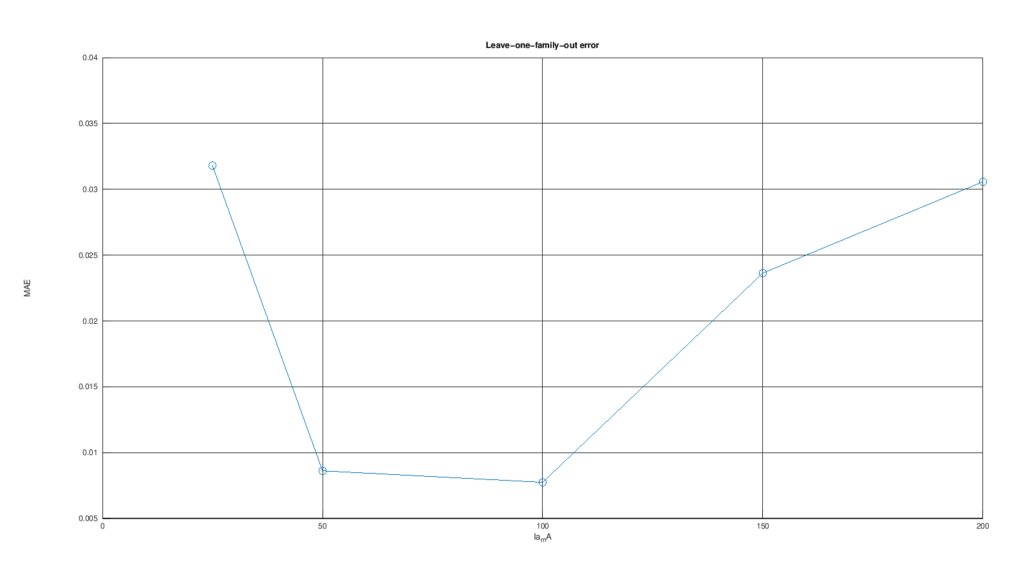
The result therefore suggests that \(V_0\) has a sufficiently regular dependence on anode current to be represented by a continuous law. In the folds at the lower edge of the interval, however, the optimizer also reported convergence problems, so the rational form must be regarded as provisional. The number of available families is also limited; this relation is therefore a promising description of the 2D21, not an already established general law.

The case of \(S_-\)

I found the behavior of \(S_-\) more difficult to describe.

The observed values do not follow a simply increasing or decreasing trend: \(S_-\) initially increases with anode current, reaches a maximum region, and then decreases.

A constant law is clearly insufficient. I therefore tried a quadratic law, the simplest available model capable of representing a rise followed by a fall: \[ S_-(I_a)=c_0+c_1I_a+c_2I_a^2. \]

When all families are used simultaneously, the quadratic curve reproduces the overall trend of the points reasonably well. The result changes, however, when I move to leave-one-family-out validation.

When one family is excluded at a time, prediction errors for \(S_-\) increase substantially. For some currents the prediction differs from the observed value by several tens of millivolts and, in the worst case, the error approaches half the actual value of the parameter.

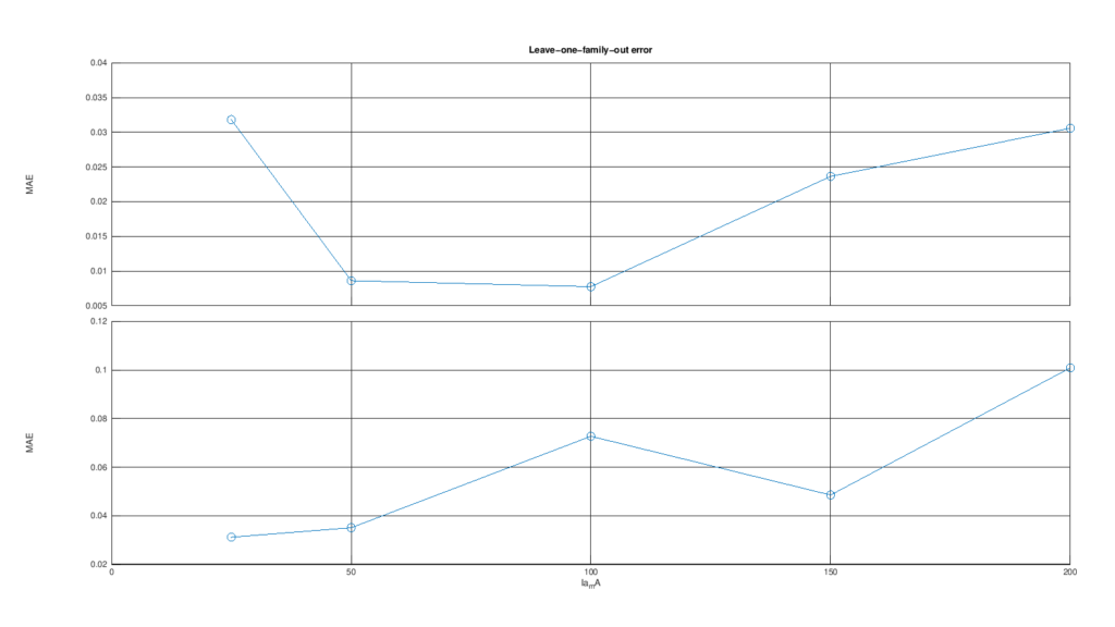
The quadratic law can represent the geometric shape of the five observed values, but the LOFO test shows that this shape is not stable enough to be used safely to derive \(S_-\) at an arbitrary anode current.

This is an important result because it shows the difference between describing the available points and predicting a point not used in the fit.

Comparison with a simple constant law did not provide a satisfactory solution either. With the data currently available, no simple and sufficiently robust continuous law for \(S_-(I_a)\) emerges.

What this means for the model

This result does not mean that the compact grid-current model is wrong.

The fundamental distinction is between the model of an individual characteristic: \[ I_g = F\!\left( V_g,I_a; V_0,S_-,S_+,Q_A,U_{20} \right) \]

and the possible laws that would automatically predict its parameters: \[ V_0(I_a),\quad S_-(I_a),\quad S_+(I_a),\quad Q_A(I_a),\quad U_{20}(I_a). \]

The first problem is the one addressed in constructing the Level-1 model: once the parameters of a family are known, the formula describes the corresponding characteristic.

The second is an additional problem: it requires the parameters themselves to follow sufficiently regular laws that they can be predicted at unobserved anode-current values.

The tests show that at least \(V_0\) has a promising structure, whereas for \(S_-\) the five available main families are not sufficient to identify a simple and robust predictive law.

Consequently, in version 0.1 the parameters \(V_0\), \(S_-\), \(S_+\), \(Q_A\), and \(U_{20}\) remain specific parameters of each individual family.

The model can therefore be used to reconstruct and analyze the characteristics for which I have determined these parameters, but I do not yet artificially extend it to a continuous surface \(I_g(V_g,I_a)\) capable of generating any intermediate anode current.

This choice is deliberately conservative. Rather than introducing more complex functions merely to interpolate five points, I prefer to keep the current model limit explicit and separate what is supported by the data from what would require further information.

It is important not to confuse this result with a negative test of the Level-1 model. In this test I am not asking \(G_-\) to reproduce a curve whose parameters I know; I am doing something more difficult, namely trying to predict those parameters using only anode current and the other available families.

The fact that \(S_-\) cannot be predicted accurately enough therefore means that a reliable \(S_-(I_a)\) law has not yet been found. It does not mean that \(S_-\), once determined from the family under consideration, fails to allow the Level-1 model to describe that characteristic correctly.

This experiment therefore establishes a precise limit of the current version: the model describes families through parameters specific to each family, but it is not yet a complete continuous model capable of deriving all those parameters automatically from \(I_a\) alone.

Physical interpretation and model limitations

So far I have built the model starting from the geometry of the curves and from their ability to collapse, at least partially, after suitable transformations. This approach makes it possible to obtain a compact mathematical description without assuming a particular microscopic mechanism in advance.

At this point, however, it is natural to ask whether the parameters introduced can be related to the physical operation of the thyratron.

It is important to distinguish clearly among three different levels:

• what is defined directly by the model and is therefore mathematically certain;
• what is compatible with the general physics of a gas-filled tube;
• what would require additional experimental data or a more detailed physical model.

What the model establishes directly

The parameter \(V_0\) is defined as the grid-voltage value at which grid current changes sign: \[ I_g(V_0)=0. \]

There is therefore no need to assign it a specific microscopic meaning immediately. In the model it simply represents the balance point between the negative-grid-current regime and the positive one.

The quantities \(S_-\) and \(S_+\), on the other hand, are voltage scales. They transform the distance from \(V_0\) into two normalized coordinates: \[ X_-=\frac{V_g-V_0}{S_-}, \qquad X_+=\frac{V_g-V_0}{S_+}. \]

Different values of \(S_-\) or \(S_+\) therefore indicate that a family must be compressed or expanded more strongly along the voltage axis to assume a shape comparable with the others.

The parameter \(Q_A\) has an equally precise definition: \[ Q_A= -\lim_{X_-\rightarrow-\infty}G_-(X_-). \]

It represents the asymptotic depth of the normalized negative branch. Similarly, \(U_{20}\) is the normalized position at which the negative branch reaches: \[ G_-(-U_{20})=-0.020. \]

These meanings are geometric properties of the model and do not depend on any particular physical interpretation.

A possible physical interpretation

During anode conduction, under the conditions represented by the GE graph analyzed in this work, the control grid is immersed in the discharge plasma. The current collected by the grid can therefore contain contributions of opposite sign associated with ions and electrons.

From this point of view, crossing \(I_g=0\) can plausibly be interpreted as a condition in which the net charge contributions collected by the grid balance one another, still during anode conduction.

This interpretation is compatible with the mathematical meaning of \(V_0\), but the present work does not identify the individual current components separately and therefore cannot establish which microscopic process determines the exact value of \(V_0\).

The normalization \[ Y=\frac{I_g}{I_a} \]

also provides an interesting indication. The fact that families obtained at very different anode currents become much more similar after division by \(I_a\) suggests that an important part of grid current grows together with the overall intensity of the conduction process in the tube.

This observation is consistent with the idea that \(I_a\) may act as an indirect measure of plasma intensity or of the population of charged particles available to contribute to grid current.

The model, however, demonstrates only the effectiveness of the normalization. It does not allow direct identification of plasma density, mobility, gas pressure, or particle energy distributions.

The positive branch

For \(V_g>V_0\), the positive master curve is described by: \[ G_+(X_+;K) = 0.005 \frac{e^{KX_+}-1}{e^K-1}. \]

The presence of an exponential dependence is qualitatively compatible with many phenomena in which electron collection depends strongly on the applied potential.

The exponential shape of the positive branch can therefore be viewed as compatible with an increasing electronic component of grid current as the grid potential becomes more favorable to electron collection.

This does not mean, however, that the parameter \(K\) can be identified directly with an electron temperature, a plasma potential, or another specific physical quantity.

In the current model \(K\) remains an empirical shape parameter of the device. Relating it to more fundamental physical quantities would require independent data that the datasheet does not provide.

The negative branch

On the negative branch, \(Q_A\) describes the approach of normalized current to a plateau.

One possible interpretation is that, as the grid becomes progressively more negative, one component of the current reaches a condition in which further changes in voltage alter the collected charge less and less.

This behavior is compatible with an ion-collection process limited by the available particle population, but the model cannot demonstrate that \(Q_A\) corresponds directly to a specific ion saturation current.

I also interpret the three exponential terms \[ e^{\lambda_1 X_-}, \qquad e^{\lambda_2 X_-}, \qquad e^{\lambda_3 X_-} \]

with caution.

I chose the three-term structure because it describes the observed curve geometry stably. The leave-one-family-out test also shows that this structure remains sufficiently stable when a single family is excluded from identification.

On the basis of the data used in this work alone, however, there is no justification for associating the three values \[ 0.060,\qquad0.240,\qquad0.960 \]

with three distinct physical processes in the tube.

I therefore regard the \(1:4:16\) progression as a compact, regularized modeling choice, not as the discovery of three fundamental thyratron constants.

Why do the two branches not have the same derivative?

The model imposes: \[ G_-(0)=G_+(0)=0, \]

but does not impose equality of the derivatives.

Mathematically, the model is therefore continuous at \(V_0\), but may show a change in slope between the negative and positive branches.

It would not be correct to interpret this result automatically as a real physical discontinuity in the device current.

More cautiously, I interpret it as an indication that the two regions of the characteristics are better described by two different compact forms. The change in slope may reflect a transition between collection regimes dominated by different contributions, or simply the limitation of a macroscopic representation obtained from static datasheet curves.

A static model, not a complete thyratron model

The model developed in this article describes only the static grid-current characteristic during anode conduction, that is, the family of curves used for its identification: \[ I_g=F(V_g,I_a). \]

It does not describe the complete dynamic behavior of the 2D21.

In particular, the current version does not include:

• the time-dependent ionization process;
• deionization after anode current is interrupted;
• the thyratron’s latch behavior after firing;
• interelectrode capacitances;
• dynamic effects of the screen grid;
• the complete conducting-state characteristic;
• explicit dependence on temperature, gas pressure, or the tube’s previous history.

These phenomena are fundamental to building a complete SPICE macromodel of the device, but they are a separate problem from the static grid-current characteristic studied here.

The role of the screen grid

Another important limitation concerns \(G_2\).

To build the model I used the curves published by the manufacturer under the conditions specified in the datasheet. These curves do not constitute a complete characterization of the dependence of grid current on the voltages applied to all electrodes.

I therefore interpret the Level-1 model within the electrical domain corresponding to the conditions of the original curves.

This point will become particularly important when I use the model to simulate the Zenith Flash-Matic remote-control receiver, because in the original circuit the 2D21 screen grid is not simply held at a fixed DC potential.

When I simulate the complete circuit I will therefore have to check how representative the characteristic derived from the datasheet remains under the actual receiver conditions.

The model does not claim to be universal

I identified version 0.1 using a single thyratron type, the 2D21.

I therefore cannot conclude that the same functions \(G_-\) and \(G_+\), the same exponential constants, or the same \(K\) value are valid for every thyratron.

A genuinely interesting test will be to apply the same procedure to different devices, initially keeping the mathematical structure frozen and observing which parameters need to change.

If several comparable thyratrons could be described with the same normalized functions and only a few device-specific parameters, the structure would acquire a much broader significance.

If, on the other hand, some classes of devices required different forms, that result would also be useful because it would help define the model’s validity domain.

What does version 0.1 represent, then?

I regard the result as a static, data-driven compact model of 2D21 grid current.

Its strength does not lie in providing a complete microscopic theory of the thyratron, but in reducing a complex family of experimental curves to a relatively simple mathematical structure, with clearly defined geometric parameters and an accuracy comparable with the uncertainty of the starting data.

Any connection between these parameters and deeper physical quantities remains an open question.

For the moment I prefer to keep the two levels separate: first I establish precisely what the model describes; then I will test whether that structure can be explained or generalized through a more fundamental physical model.

The complete Level-1 model

At this point I can collect the model obtained for 2D21 thyratron grid current into a single form.

The first transformation is the normalization of grid current to anode current: \[ Y=\frac{I_g}{I_a}. \]

For each family I then identify the value \(V_0\) for which: \[ I_g(V_0)=0. \]

I treat the two sides of the characteristic separately using two voltage scales: \[ X_-=\frac{V_g-V_0}{S_-}, \qquad V_g\leq V_0, \]

and \[ X_+=\frac{V_g-V_0}{S_+}, \qquad V_g\geq V_0. \]

Positive branch

For \(V_g\geq V_0\), normalized current is described by the master curve: \[ \boxed{ G_+(X_+;K) = 0.005\, \frac{\exp(KX_+)-1} {\exp(K)-1} } \]

with: \[ \boxed{K=0.551}. \]

The factor \(0.005\) follows from the convention used to define the scale \(S_+\): \[ G_+(1)=+0.005. \]

Positive grid current is therefore: \[ \boxed{ I_{g,+} = I_a\, 0.005\, \frac{ \exp\!\left[ K\frac{V_g-V_0}{S_+} \right]-1 }{ \exp(K)-1 } } \]

for \(V_g\geq V_0\).

Negative branch

For \(V_g\leq V_0\), the normalized function takes the form: \[ \boxed{ G_-(X_-;Q_A,U_{20}) = -Q_A+ \sum_{j=1}^{3} A_j e^{\lambda_j X_-} } \]

with the three constants: \[ \boxed{ (\lambda_1,\lambda_2,\lambda_3) = (0.060,\;0.240,\;0.960) }. \]

The coefficients \(A_1\), \(A_2\), and \(A_3\) are not free parameters. I determine them by imposing: \[ G_-(0)=0, \] \[ G_-(-1)=-0.010, \]

and \[ G_-(-U_{20})=-0.020. \]

Consequently: \[ \begin{bmatrix} 1 & 1 & 1 \\ e^{-\lambda_1} & e^{-\lambda_2} & e^{-\lambda_3} \\ e^{-\lambda_1U_{20}} & e^{-\lambda_2U_{20}} & e^{-\lambda_3U_{20}} \end{bmatrix} \begin{bmatrix} A_1\\ A_2\\ A_3 \end{bmatrix} = \begin{bmatrix} Q_A\\ Q_A-0.010\\ Q_A-0.020 \end{bmatrix}. \]

Negative grid current is therefore: \[ \boxed{ I_{g,-} = I_a \left[ -Q_A+ \sum_{j=1}^{3} A_j \exp\!\left( \lambda_j \frac{V_g-V_0}{S_-} \right) \right] } \]

for \(V_g\leq V_0\).

Complete form

The static compact model can therefore be written in piecewise form as: \[ \boxed{ I_g(V_g,I_a)= \begin{cases} I_a\, G_-\!\left( \dfrac{V_g-V_0}{S_-}; Q_A,U_{20} \right), & V_g\leq V_0, \\[12pt] I_a\, G_+\!\left( \dfrac{V_g-V_0}{S_+}; K \right), & V_g\geq V_0. \end{cases} } \]

The two branches satisfy: \[ G_-(0)=G_+(0)=0, \]

so current remains continuous at \(V_0\). I do not impose derivative continuity.

Parameters identified for the 2D21

The following table summarizes the parameters obtained for the main families used in constructing and checking the model.

\(I_a\)	\(V_0\)	\(S_-\)	\(S_+\)	\(Q_A\)	\(U_{20}\)
25 mA	-0.28418 V	0.14187 V	0.03058 V	0.03136	4.995
50 mA	-0.36110 V	0.23812 V	0.04413 V	0.02802	3.746
100 mA	-0.43804 V	0.25758 V	0.06747 V	0.02819	4.984
150 mA	-0.45898 V	0.32066 V	0.05269 V	0.02884	4.072
200 mA	-0.50980 V	0.21483 V	0.05017 V	0.03254	4.592
300 mA	-0.57868 V	0.07533 V	≈0.014 V	0.04810	4.473

The value of \(S_+\) at 300 mA requires particular caution: the digitized curve does not reach the \(Y=+0.005\) level used to define this scale directly, so the reported value is inferred from the model.

\(Q_A\) for the 300 mA family is also less directly determined than for the other families because the available characteristic does not extend far enough into the negative region to show the plateau completely.

I do not include the 5 mA family in the main table because it behaves differently and I keep it as a possible low-current regime. The same negative-branch structure can nevertheless describe it with \(Q_A\approx0.044\) and \(U_{20}\approx3.07\).

What the model can do — and what it cannot do yet

The result compresses a family of \(I_g(V_g)\) characteristics into a small set of geometric parameters.

For a family for which \[ V_0,\qquad S_-,\qquad S_+,\qquad Q_A,\qquad U_{20}, \]

are known, a continuous grid-current characteristic can be reconstructed without using the original series of digitized points directly.

It has not yet been demonstrated, however, that all of these parameters can be calculated reliably from anode current \(I_a\) alone.

An initial test of the current dependence of the parameters showed that \(V_0\) has a promising regularity, whereas \(S_-\) cannot yet be predicted robustly by a simple continuous law.

This means that I do not interpret version 0.1 as an already complete continuous surface: \[ I_g=F(V_g,I_a) \]

capable of automatically generating a characteristic at any arbitrary anode current.

At present, the verified level is more precisely: \[ \left( V_0,S_-,S_+,Q_A,U_{20} \right) \longrightarrow I_g(V_g). \]

Determining laws that connect these parameters to \(I_a\) is a subsequent problem, and I keep it separate from the Level-1 model.

Conclusions

The initial objective of this work was very practical: to obtain a usable model of 2D21 grid current starting from the original GE datasheet curves, rather than relying on an online macromodel whose parameter origin was not clear.

The process turned out to be broader than expected.

I digitized the original characteristics several times, compared them across independent acquisitions, and transformed them into consensus curves accompanied by an uncertainty estimate.

Analysis of the normalized curves then showed that a substantial part of their apparent complexity can be separated into a few elements:

• a zero-crossing point \(V_0\);
• two voltage scales \(S_-\) and \(S_+\);
• a positive master curve characterized by the parameter \(K\);
• a common negative structure corrected by two geometric parameters,
  \(Q_A\) and \(U_{20}\).

The result is a relatively simple static piecewise compact model, continuous at the grid-current sign-change point and capable of describing the main families with errors of the same order as the dispersion present in the digitized data.

Several tests also made it possible to verify that the structure does not simply depend on the large number of points used to represent the curves. When I greatly reduce the grid density, the main parameters remain essentially unchanged.

The work also revealed precise limitations.

The 5 mA family may represent a different regime; some parameters of the 300 mA family are less directly identifiable; derivative continuity at \(V_0\) is not supported by the data; and it is not yet possible to derive all model parameters reliably from anode current alone.

Most importantly, this is not yet a complete thyratron model.

It does not describe ionization, deionization, latch behavior, interelectrode capacitances, time-domain dynamics, or the complete behavior after firing. I will add these elements separately when I transform the model into a SPICE component intended for circuit simulation.

The result of version 0.1 is therefore deliberately more limited: a quantitative and reproducible model of the static 2D21 grid-current characteristic, derived directly from the manufacturer’s curves.

The next step: returning to the Flash-Matic

This work began as a necessary detour during the reconstruction of the Zenith Flash-Matic remote-control receiver.

In the original circuit, the 2D21 is not used as a simple ideal switch. Its firing depends on the signal produced by the photocells and on the electrical conditions applied to the grids, while after firing the tube’s conduction, latch behavior, and subsequent recovery come into play.

The model developed in this article describes only one of these parts: control-grid current during anode conduction. By itself, therefore, it is neither a model of the Flash-Matic trigger nor of the region preceding firing.

The next step will be to implement this static law as a sub-block of the SPICE model and add the other required characteristics: pre-conduction behavior, second-grid dependence, triggering, latch behavior, extinction, and recovery.

At that point I will finally be able to return to the Flash-Matic schematic and study not only whether the circuit works in simulation, but also how sensitive it was to useful light, ambient light, and real component tolerances.

In other words, the 2D21 model is not the endpoint of the project: it is one of the tools needed to answer the question from which the entire investigation began.

Downloadable data and material

To make the analysis reproducible, I make the data and files used to construct the model available together with the article.

• Consensus-curve dataset used for fitting
• 2D21 Level-1 parameter table
• Mathematical specification of the Level-1 v0.1 model
• Uncertainty data from replicated digitizations

I will add the future SPICE implementation separately after numerically verifying the correspondence between the analytical law and the simulatable model. This will keep the original mathematical model clearly distinguishable from its circuit implementation.