GX-TXT Curve Digitalizer — Guide 03: Digitizing Log-Log Plots

From a raster image to a verifiable Dataset: the example of the function y = √x

Not all axes in scientific plots are linear. When a quantity spans several orders of magnitude, a logarithmic scale is often preferable: equal distances on the chart represent equal ratios between values, not equal differences. This changes how an image must be calibrated and makes it risky to convert pixels directly using a simple linear proportion.

In this third guide, we use GX-TXT Curve Digitalizer to recover data from a synthetic chart with two logarithmic axes. We know the function in advance, y = √x, so we can distinguish what is mathematically known from what the digitizer actually measures on the raster. We will follow the complete workflow: importing, calibrating, verifying, placing guide points, assisted tracing, publishing the Dataset and checking it in Preview.

1. Our sample: a known function on a log-log chart

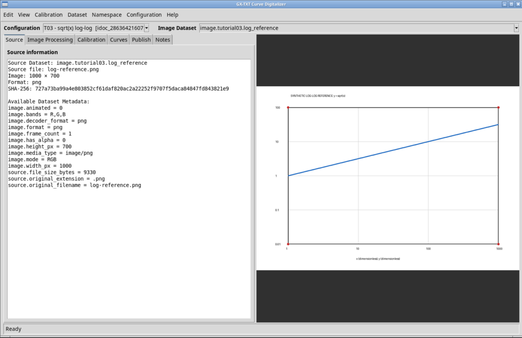
The starting image, log-reference.png, is a 1000 × 700 pixel RGB raster. The blue line represents y = √x; the four red markers define the rectangle used for calibration. The reference axis values are:

Axis	Minimum	Maximum	Scale	Unit
X	1	1000	Logarithmic	1 (dimensionless)
Y	0.01	100	Logarithmic	1 (dimensionless)

On a log-log plot, the function appears as a straight line because log₁₀(y) = 0.5 · log₁₀(x). The expected slope in logarithmic coordinates is therefore 0.5. This follows from the function and the choice of axes; it is not a result of digitization.

For concrete reference points, the theoretical curve contains (1, 1), (10, 3.1623), (100, 10) and (1000, 31.6228). We will not use these values to generate the data artificially: we will retain them as independent comparison references.

2. Importing the source as a Dataset

We create a new GX-TXT Session, separate from the experiments in the previous guides. In Acquisition, we select Image importer, choose log-reference.png, assign the ID image.tutorial03.log_reference and import the file.

Importing creates a canonical Dataset with the image.raster contract. Curve Digitalizer can then work with a source linked to the Session, without relying on private paths or manually replacing images inside the project.

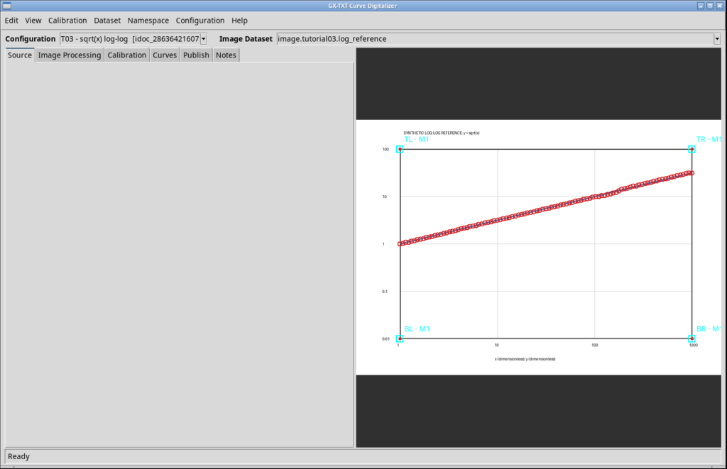
We open Viewers → Digitalizer, create a new configuration named T03 - sqrt(x) log-log, select the newly imported Dataset under Image Dataset and confirm the preview dialog with Use this image. The Source panel displays the source identity, raster dimensions and SHA-256 fingerprint.

3. Setting both axes to logarithmic scale

In the Calibration tab, we configure X and Y before selecting the reference points. For X, we enter label x, unit 1, semantic role independent, minimum 1, maximum 1000, and Scale = log. For Y, we enter label y=sqrt(x), unit 1, role measured, minimum 0.01, maximum 100, and again Scale = log. We leave the Y direction at Upward (Cartesian) and click Apply axis settings.

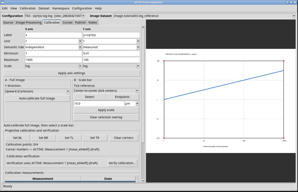
A logarithmic scale requires strictly positive limits. During the test, we also checked the interface by temporarily entering Y minimum = 0: the Digitalizer rejected the setting with the warning “Logarithmic axes require positive limits.” We then restored the correct minimum, 0.01, without changing the valid calibration.

4. Calibrating the four corners of the raster

The image uses manual four-point calibration. In the same Calibration tab, we select Set BL, Set BR, Set TL, and Set TR in that order, clicking the corresponding red markers: bottom left, bottom right, top left and top right.

The points actually recorded during the GUI test, expressed in the original image’s pixel coordinates, are:

Corner	Pixel X	Pixel Y
BL	119.424	599.640
BR	919.424	599.640
TL	119.424	80.216
TR	919.424	80.216

The values do not match the nominal marker centers (120, 600), (920, 600), (120, 80), and (920, 80) exactly: they are coordinates obtained from actual clicks on the canvas, at finite display resolution. The system recognized the calibration, and we changed Measurement 1 from draft to accepted.

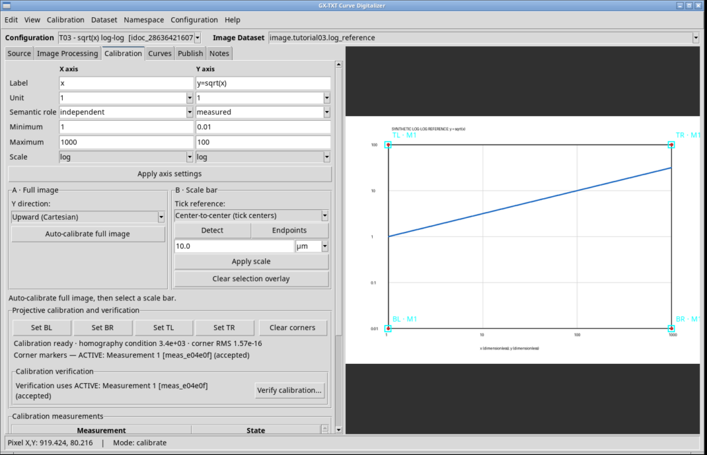
The Digitalizer reported a homography condition number of approximately 3.4 × 10³ and a four-corner reprojection RMS of approximately 1.57 × 10⁻¹⁶. This RMS describes how consistently the transformation reproduces the points used to calculate it: it is not the uncertainty of the digitized curve and does not, by itself, demonstrate digitization accuracy.

5. Checking known reference points

We use Verify calibration… to select identifiable points on the blue trace, entering the function’s expected physical coordinates in the Expected fields. The interface returns the coordinates calculated from calibration and their deviations, without modifying the Dataset.

Theoretical X	Theoretical Y	GUI X	GUI Y
1	1	1.0000	1.0128
10	3.1623	10.0832	3.1927
100	10	100.4150	10.0640
1000	31.6228	1000.0000	31.7238

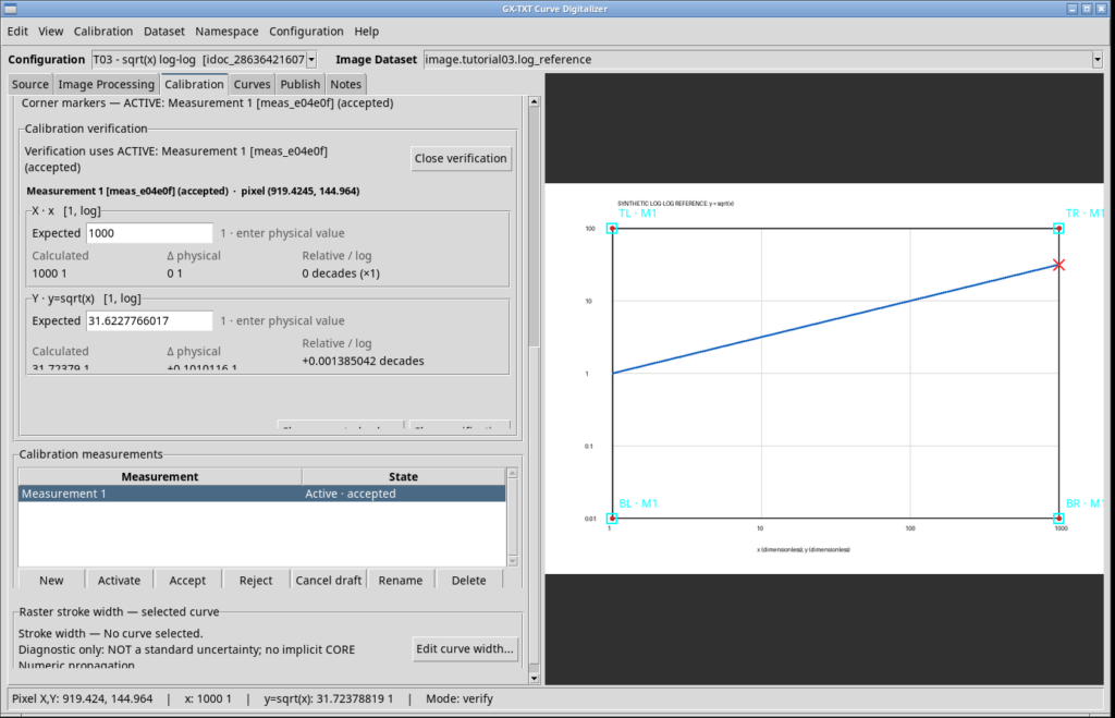
The deviations are small relative to the overall range, but they are not zero. Pixel selection, line thickness, marker placement and image resampling all limit practical precision. The interactive check described here must not be confused with a complete metrological uncertainty assessment.

6. Tracing the curve with five guide points

We switch to the Curves tab. We are not building a curve family, so we leave This configuration is a numerical curve family unchecked and create a single curve using New curve, naming it sqrt(x).

For the assisted tracing test, we enable Add guide and place five points along the blue line, from its first to its last endpoint. The guide points describe the intended path; they are not yet the one hundred points we will publish.

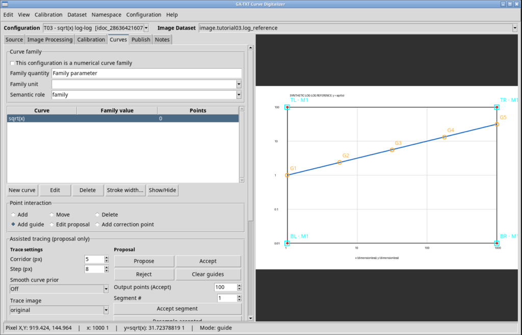
We set Corridor = 5 px, Step = 8 px, Smooth curve prior = Off and Trace image = original. In the acceptance controls, we specify Output points (Accept) = 100. Clicking Propose, Curve Digitalizer generates a proposal of 105 points across 4 segments; in this test it reports no ambiguous segments in the proposal. We visually inspect the overlay before continuing.

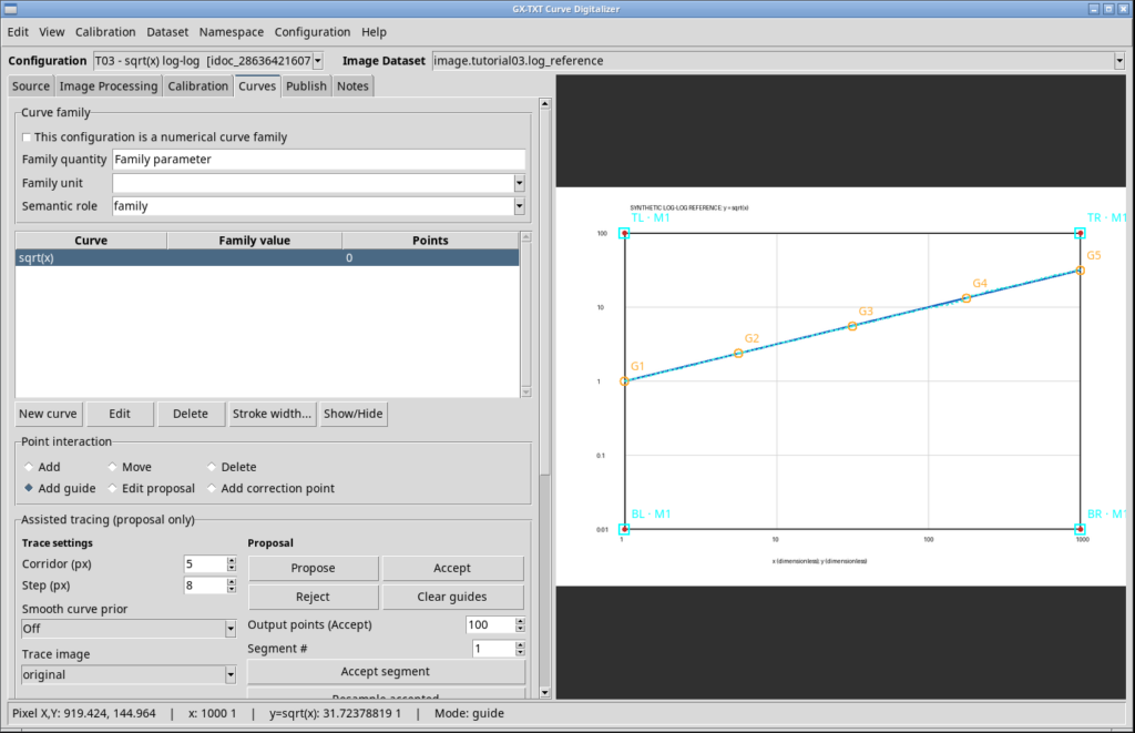
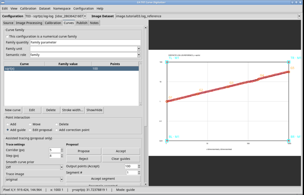
With Accept, we confirm the four segments. The interface reports 100 assisted points added. The final curve contains 100 points. The difference between 105 proposed points and 100 accepted points results from the selected output density, not from the accidental loss of five data points.

7. Publishing the canonical Dataset

In the Publish tab, we enter digitized.tutorial03.sqrt_loglog as the base name, select the separate layout and choose the only accepted calibration measurement, Measurement 1. We click Publish selected calibrations.

The result is a canonical Dataset with the following ID:

digitized.tutorial03.sqrt_loglog.measurement_1.curves

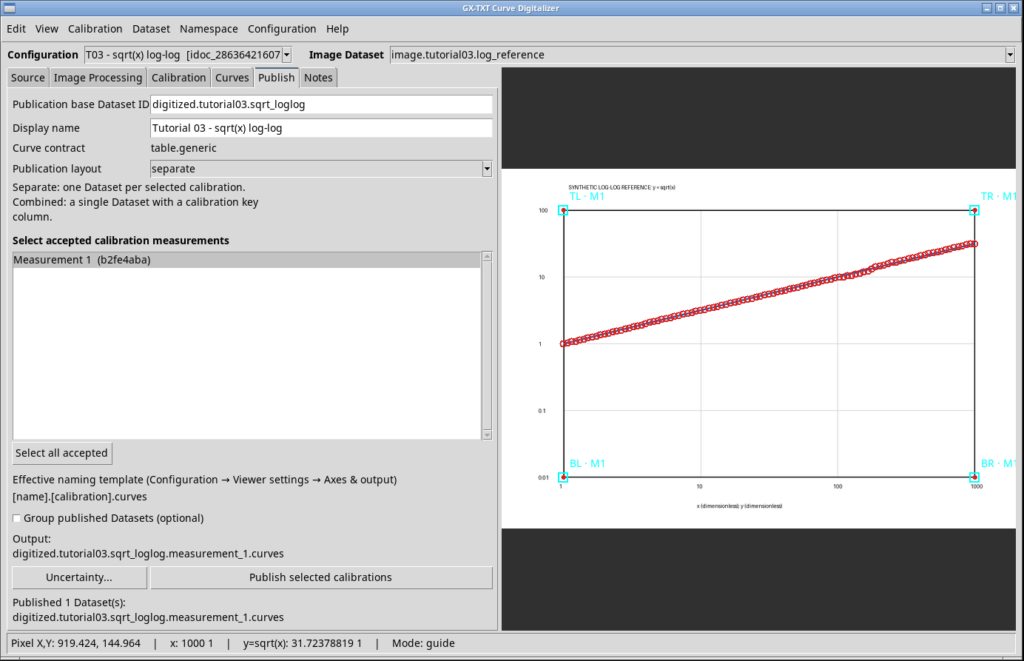
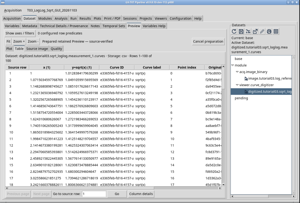
The published Dataset contains 100 rows and eight columns: x, y, curve_id, curve_label, point_index, point_id, pixel_x, and pixel_y. The first two contain scientific coordinates; the last two preserve positions in the original raster. Identifiers and indices link the rows to their source curve and points. We have not produced multiple copies of the same points through alternative calibrations.

8. Checking the results in Dataset Preview

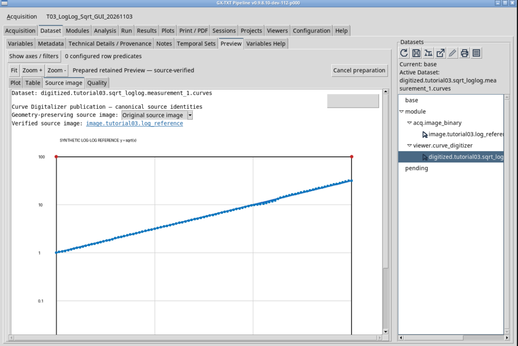
In the GX-TXT Dataset panel, we activate the new Dataset and open Preview. The available tabs include Source image, Plot, Table and Quality.

The Source image tab displays the original chart with the digitized points overlaid. This provides the most immediate visual check of whether the trace remained on the blue line.

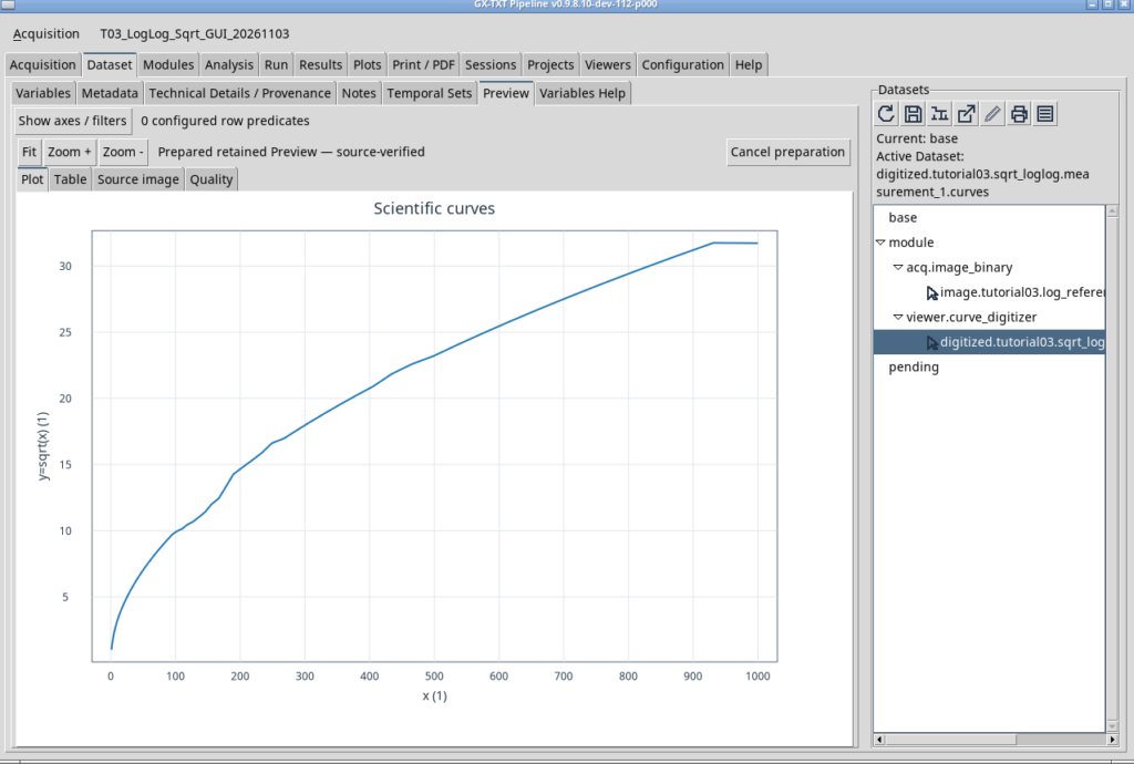
The Plot tab, by contrast, displays the numerical X and Y values stored in the Dataset. In our test, the initial view uses linear presentation axes. The function therefore has its familiar square-root shape, rather than appearing as the straight line seen on the original log-log chart.

In the Table tab, we find all 100 rows of the Dataset, including scientific coordinates and references to the original raster pixels.

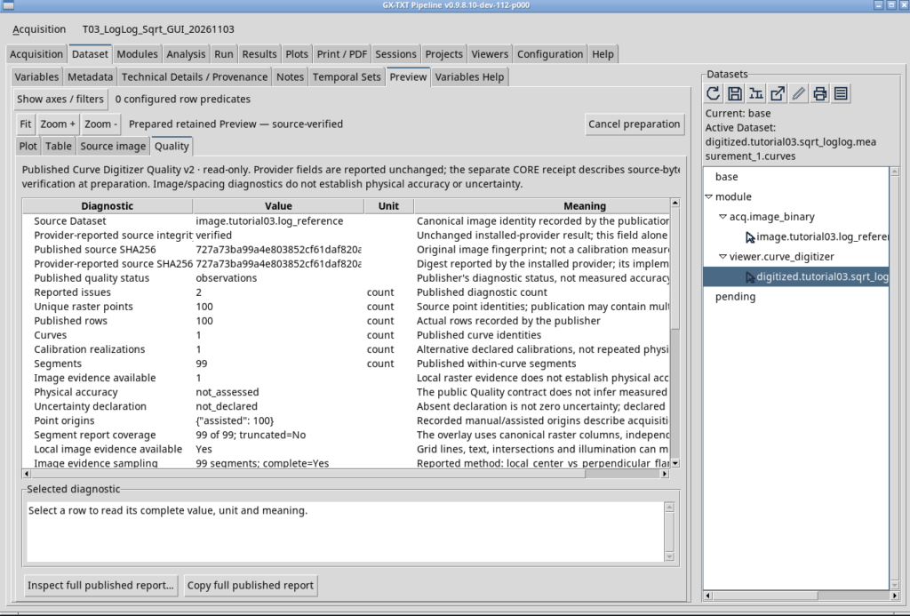
Finally, Quality displays the publication’s diagnostic report. In our case, it shows one curve, 100 raster points, 99 segments and two informational observations of weak local contrast. These do not automatically indicate two incorrect points, nor do they constitute an estimate of physical error. The report distinguishes image observations from metrological accuracy and uncertainty, neither of which was assessed or declared.

9. How closely do the points match the theoretical function?

Because we know the model, we can perform a numerical check independent of the screenshot using the published CSV. For each row, we take the digitized X, calculate the theoretical square root of that same X and compare it with the digitized Y. The percentage relative deviation is:

100 · [Y(digitized) − √X(digitized)] / √X(digitized).

For the 100 points actually published, we obtained:

Metric	Result
Points compared	100
RMS relative error versus y = √x	2.395%
Maximum absolute relative error	5.489%
Slope of log₁₀(Y) versus log₁₀(X) regression	0.503632
Intercept of the same regression	−0.002120

The fitted slope of 0.5036 is close to the theoretical slope of 0.5. This confirms that the data broadly follow the expected relationship. It does not mean that every point is correct: local deviations, especially with a trace only a few pixels thick, must be examined separately.

The 2.395% RMS value describes how much the Dataset differs from the reference function in this synthetic exercise. It is not a standard uncertainty that can automatically be assigned to new measurements, nor an indication of the digitizer’s universal performance on arbitrary images.

10. Saving, closing and reopening

We finish by saving the configuration in the Session. We close Curve Digitalizer and reopen it via Viewers → Digitalizer, without recreating the source or repeating the import. The same T03 - sqrt(x) log-log configuration is restored together with the image, calibration and all 100 accepted points.

Conclusion

This experiment demonstrates the complete workflow from a scientific image to a traceable numerical Dataset. The important aspects are not just tracing speed but, above all, correct interpretation of the scales, verification against known points, preservation of raster coordinates and a clear distinction between published data, image diagnostics and physical uncertainty.

The function y = √x is a particularly useful teaching example: it is a straight line on the log-log raster, while it returns to its square-root shape in a linear numerical representation. The scientific content of the data remains unchanged; only the way we choose to display it differs.

Materials for reproducing the experiment

To repeat the experiment, you need the original image log-reference.png. The companion file log-reference.json describes the ideal geometry and mathematical reference values. These are useful for comparison but do not replace calibration carried out in the GUI. Both files are included in the teaching materials package