Digitizing Datasheet Curves in GX-TXT: the Curve Digitizer Viewer

15 October 2026 di giux Electronics, Featured, GX-TXT 8 min di lettura

From a standalone program to a GX-TXT viewer

In the GX-TXT introduction I said I would go through the individual tools. I am starting with the Curve Digitizer, because that is where much of my data enters the framework: curves from old datasheets that exist only as drawings.

The Curve Digitizer already exists as a standalone program: you open the image, calibrate the axes, click on the curve and leave with a CSV. Inside GX-TXT the same job changes nature. The image is not opened from a file: it is a Dataset imported into the Session. The digitization work is not a project file: it is Session state. The result is not a CSV to keep in a folder: it is a Dataset with its provenance, which plots, the fitter and the other modules read without reopening the digitizer.

The calibration model is the one from the original program, four points and a projective transform. Almost everything around it has changed.

Video presentation of the Curve Digitizer (9 minutes), generated with Gemini Notebook from the manual and the GX-TXT documentation.

Version and status

The viewer will ship in release 0.9.8.10-dev-98 and is also compatible with dev-96. It is not 100% complete, but barring bugs this is the version the framework will be released with. The manual attached at the end describes version 1.2.17 of the viewer.

No workspaces: you work with configurations

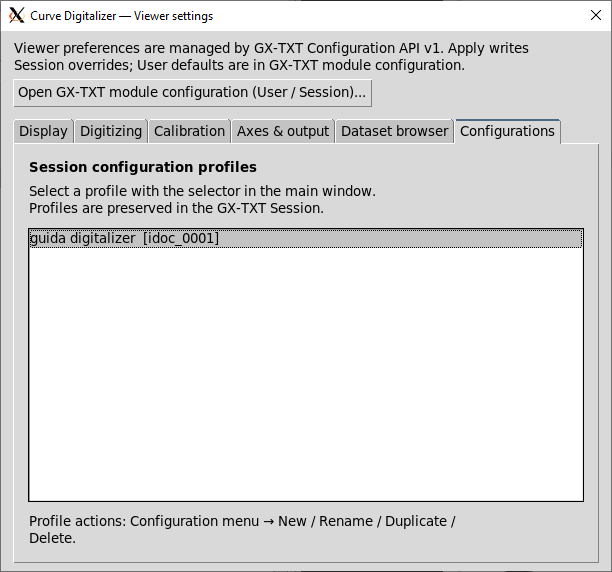
This is the first thing to know if you already use GX-TXT: the Curve Digitizer does not support workspaces. It uses configurations instead.

A configuration is the digitizer’s work object, and it ties a single source image to everything built on top of it:

the source Dataset ID and the SHA-256 fingerprint of its bytes;
the X and Y axis definitions: label, unit, semantic role, minimum, maximum, linear or log scale;
the calibration measurements;
the curves and their points, in the order they were taken;
the curve family definition, if any;
publication settings and notes.

Each configuration has a name and a stable ID, and is stored in the Session as an interactive document. Close GX-TXT, reopen the Session, reopen the viewer and pick the configuration from the selector at the top: there is no separate project file to save. The Configuration menu creates, renames, duplicates and deletes them; deleting a configuration does not delete Datasets already published.

The same image can back several independent configurations. A datasheet page with plate characteristics, transfer characteristics and grid current becomes three configurations, each with its own calibration and output Dataset. The reverse is blocked: a calibrated configuration cannot be moved to another image, because the calibration only holds for those pixels. A new image gets a new configuration.

One warning to avoid confusion: the viewer also has a Namespace menu. It filters image Datasets by organizational group; it is not a workspace, and changing the filter does not change a configuration’s source.

Curve Digitizer Viewer settings window, Configurations page listing the configurations stored in the Session — The Configurations page of the viewer settings: configurations are stored in the Session and selected from the main window.

The workflow in short

Import the image (PNG, JPEG, BMP or TIFF) with GX-TXT image acquisition: it becomes an image.raster Dataset.
Open the Curve Digitizer from the Viewers menu, create a configuration and choose the image.
Declare the axes: name, unit, role, minimum, maximum, scale.
Click the four corners of the plot area and check the calibration on a known point.
Create the curves, with the parameter value if they form a family, and click the points.
Write the notes and publish: the result is a GX-TXT Dataset.

Calibration: four corners and an independent check

Axes can be linear or logarithmic in all four combinations; a log axis needs positive limits. The four corners (bottom-left, bottom-right, top-left, top-right) define a homography, so a skewed or slightly perspective scan is calibrated without straightening it first.

When the viewer says the calibration is ready, it only means the transform is geometrically valid. The real check is Verify calibration: click a grid intersection with known coordinates, type the expected values, and the viewer reports the computed values and the residuals. In the manual’s example, at (1 V; 2 mA) the residuals are −0.012 V and −0.027 mA. Verification does not change the calibration.

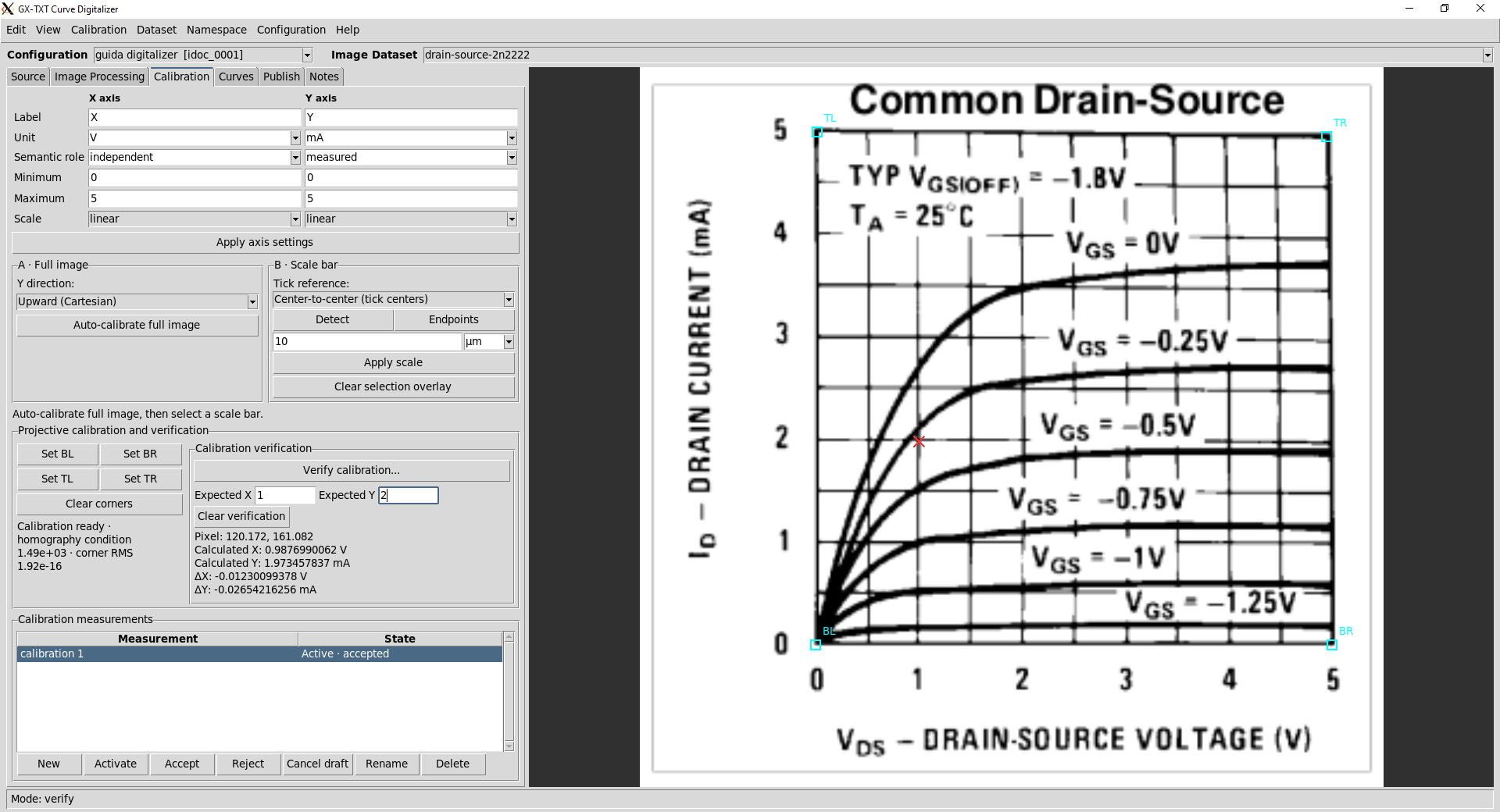
Curve Digitizer Calibration tab with a check on a grid intersection: computed values and residuals — Calibration check: the red X marks the evaluated pixel; on the left, computed values and residuals against the expected ones.

Calibration can be repeated without touching the points already taken. Each new choice of the four corners is a measurement of its own, with its own ID, label and fingerprint, and can be accepted, rejected or made active. Several calibrations of the same plot show how much hand placement of the corners matters. The viewer does not turn that spread into an uncertainty: it computes no averages and invents no error bars.

Curve families

When curves differ by a numeric parameter, such as V_GS for a FET or grid voltage for a tube, you enable family mode: declare the parameter quantity and unit, and each curve gets its value. The result is published with the curve_family.table contract, which the fitter and other modules recognize as a family. If the curves merely share a plot without a common parameter, family mode stays off.

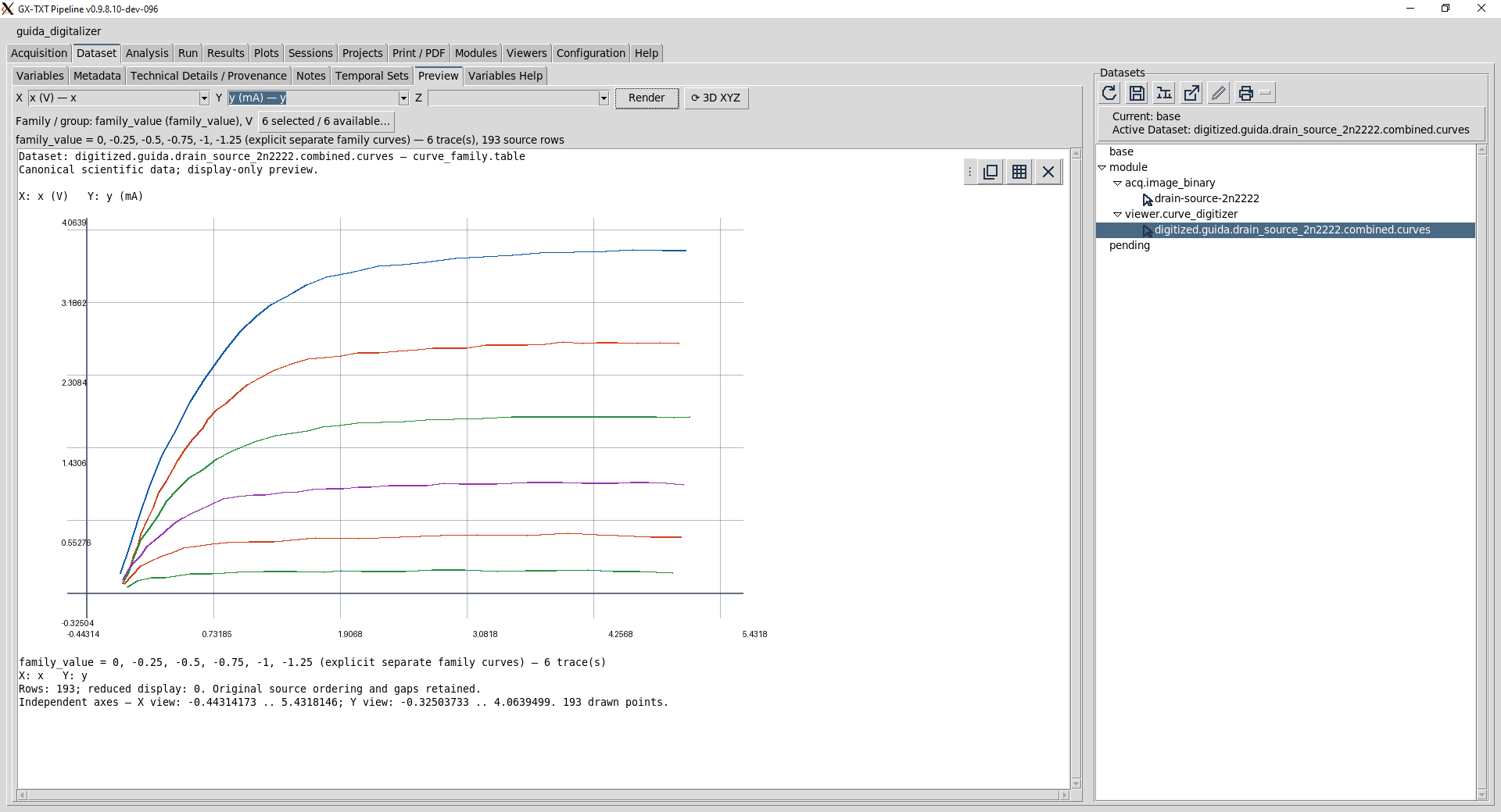
In the manual’s first example, the six I_D–V_DS curves of a datasheet, with V_GS from 0 to −1.25 V, yield 193 points.

A note on the manual. The manual attributes this curve family to the 2N2222, which is wrong: the 2N2222 is a bipolar transistor, while these are the characteristics of a FET, with V_DS, V_GS and a V_GS(off) of −1.8 V. The plot was picked practically at random and is only an example of the workflow; the name 2n2222 in the Dataset IDs shown in the screenshots comes from that.

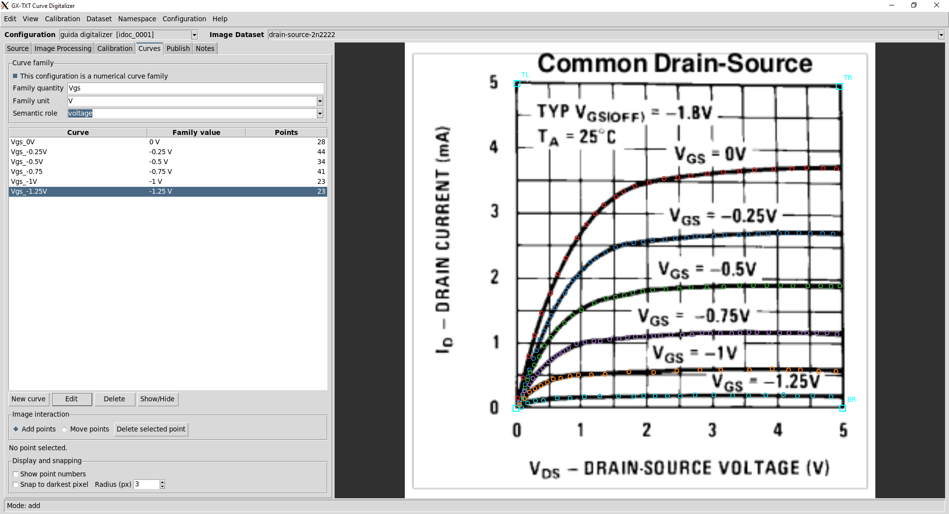
GX-TXT Curve Digitizer, Curves tab: a family of six ID-VDS curves at constant VGS digitized from a datasheet — The complete family: six curves, each with its V_GS value and point count.

Points are taken by hand, in natural X order, more densely where the curve bends. A point that landed on the grid instead of the trace is moved with Move points, without restarting the curve. Darkest-pixel snapping is available, but it is a local aid: on a scan with a thick grid it can catch the wrong line.

Publishing: a Dataset, not a CSV

In the Publish tab you choose which accepted calibrations to publish and the layout:

separate: one Dataset per calibration. It is the default and works with any module that reads X and Y;
combined: a single Dataset with all calibrations, distinguished by a key column. Only useful to consumers that handle that extra dimension.

Dataset IDs come from a naming template, [name].[calibration].curves by default, with a preview before publishing. Each Dataset carries the calibration manifest (exact homography, calibration type, axes, source with its SHA-256), written in the same transaction as the data, and keeps the original pixel coordinates of the points. Configuration notes are appended to the published Dataset’s notes.

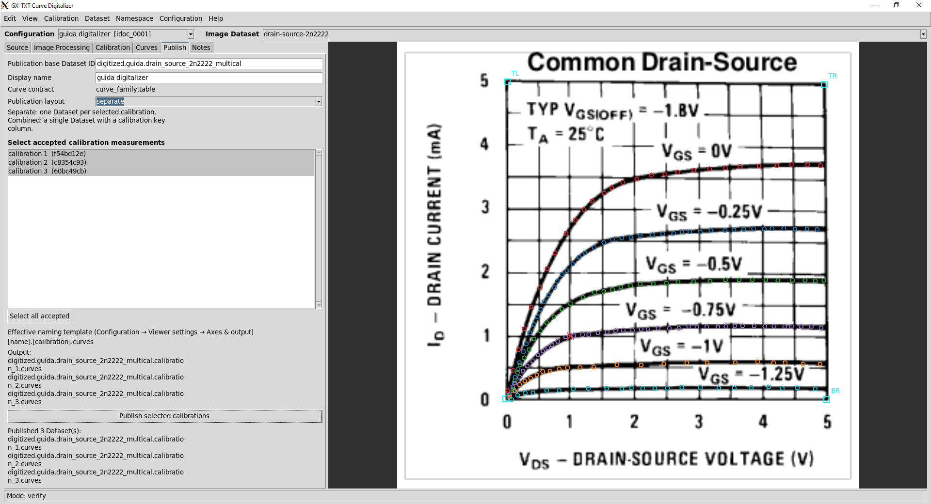
Curve Digitizer Publish tab: three calibrations in separate layout with a preview of the Dataset IDs — Publishing in *separate* mode: three calibrations of the same plot, three Datasets named by the template.

The published Dataset is data like any other: the framework’s Dataset Preview plots the family without knowing it came from a digitizer.

GX-TXT Dataset Preview plotting the six curves of the family published by the Curve Digitizer — The published family, opened in GX-TXT Dataset Preview without going through the digitizer.

If the image changes

A calibration only holds for the pixels it was made on. That is why the configuration records the image SHA-256 and checks it again every time it is opened. If the bytes changed, the source becomes STALE SOURCE: points and calibrations are kept, but editing and publishing are blocked. If the Dataset no longer exists, it becomes SOURCE MISSING, and the configuration is still kept. In no case does the viewer silently attach an old calibration to a different image.

Photographs and SEM images

The second part of the manual works on a synthetic SEM-style image of a metal microcrack, made for the exercise: it is not a real measurement. There are no printed axes here. Auto-calibrate full image calibrates the whole image in pixels, then you detect the scale bar (10 µm in the example), automatically or by marking its two ends, and apply the physical scale. Scale is assumed equal in X and Y.

To see edges better there is image processing: levels, gamma, local contrast (CLAHE), denoising, sharpening, threshold. Only operations that leave geometry alone (no crop, rotation or perspective correction), so the calibration stays valid. Original and processed images are compared side by side, and the processed image can be published as a Dataset of its own, with the filter sequence and parameters in its metadata.

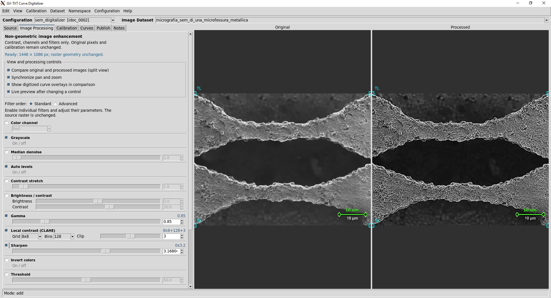
Original and processed synthetic SEM micrograph side by side in the Curve Digitizer, with a 10 µm scale bar — Original on the left, processed on the right: grayscale, auto levels, gamma, CLAHE and sharpening. Geometry does not change.

Making an edge sharper does not make it more accurate: processing helps the eye, not the measurement.

What it does not do

it does not recognize curves on its own or read the text on the plot: no automatic tracing, no OCR. The person digitizing chooses the points;
it does not open files directly: the image must first be a Session Dataset;
it does not support workspaces: you work with configurations;
it needs a Tk display (local desktop or X11 forwarding);
plots and fits on published Datasets depend on the modules that use them, normally with GNU Octave.

The manual

The illustrated manual is in English, 77 pages, version 1.2.17. It contains two complete procedures with real screenshots (a datasheet curve family and the SEM image), a reference for every viewer setting, the module’s full internal manual and the specifications of the three public APIs: calibration, curve Dataset schema, image processing.

Download the Curve Digitizer manual (PDF, 9 MB)

GX-TXT source code is on GitHub: giuxlab-hub/GX-TXT. If you try the digitizer, I want to know what works, what breaks and what is missing for your work.

#characteristic curves #curve digitization #data analysis #GX-TXT