GX-TXT Curve Digitalizer: From Botanical Micrographs to Morphometric Analysis with Python

In this guide, we use GX-TXT to extract quantitative information from an optical micrograph of plant tissue. The experiment covers micrometre-scale calibration, digitization of the outlines of four stomata, and subsequent geometric analysis using the Python editor integrated into the framework.

Curve Digitalizer is responsible solely for acquiring coordinates. Area and perimeter calculations, along with contour interpolation, are performed by a Python script using the public GX-TXT APIs.

1. Materials and objectives

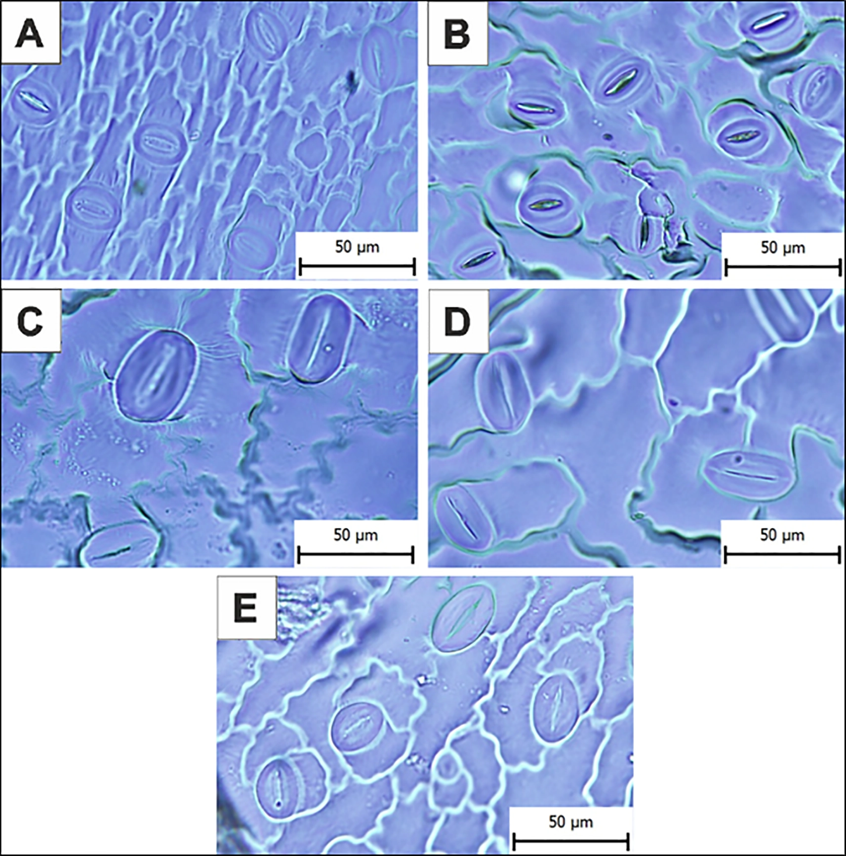
The micrograph used in this experiment comes from an article published in Frontiers in Plant Science, DOI 10.3389/fpls.2025.1676435.

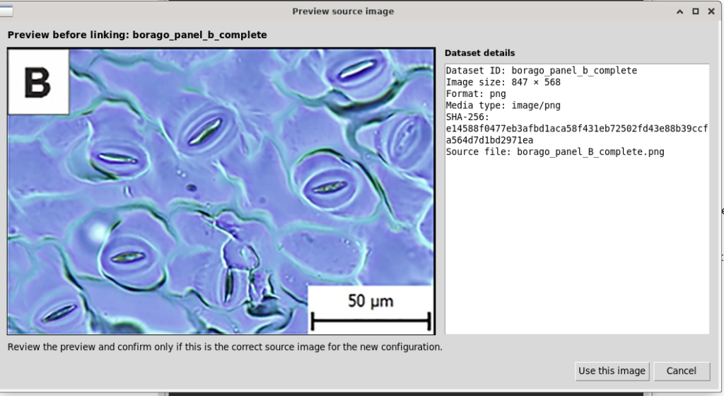
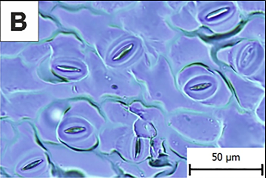
We selected panel B, showing stomata of Borago officinalis, while retaining the 50 µm reference scale bar.

The image file used for the experiment is borago_panel_B_complete.png, measuring 847 × 568 pixels.

The objective is to digitize two outlines for each stoma: the outer boundary of the stomatal apparatus and the boundary of its central opening, or stomatal pore.

These coordinates will then be used to calculate areas and perimeters, consistently distinguishing the acquired data from interpolated mathematical representations.

2. Creating the session and importing the image

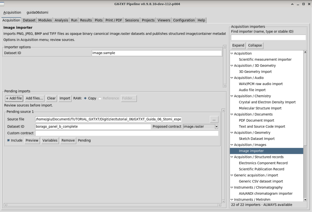
From Acquisition → Image importer, we imported the micrograph as a Canonical Image Dataset and assigned it the identifier borago_panel_b_complete.

We then opened Viewers → Digitalizer, created the stomi06 configuration, and explicitly associated it with the Image Dataset.

Checking the preview allowed us to verify the integrity of the source before proceeding with calibration.

3. Geometric calibration

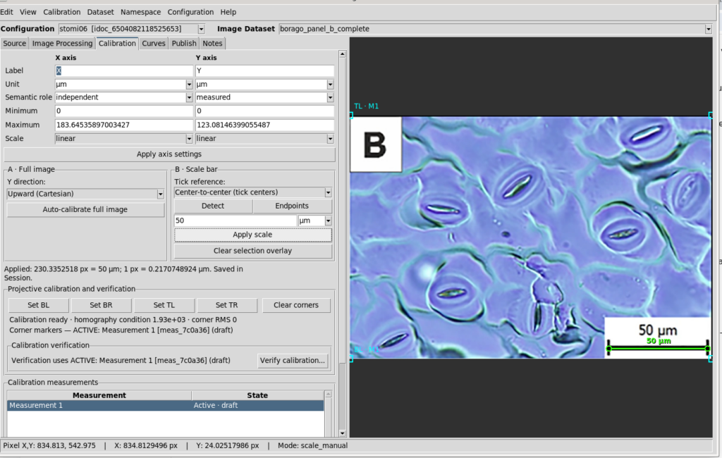
To convert image coordinates into physical quantities, we used the micrometre scale bar shown in the micrograph.

In the Calibration tab, we selected full-image calibration, set both axes to linear, and kept the Y axis increasing upwards.

Using Scale bar → Endpoints, we identified the two endpoints of the 50 µm scale bar.

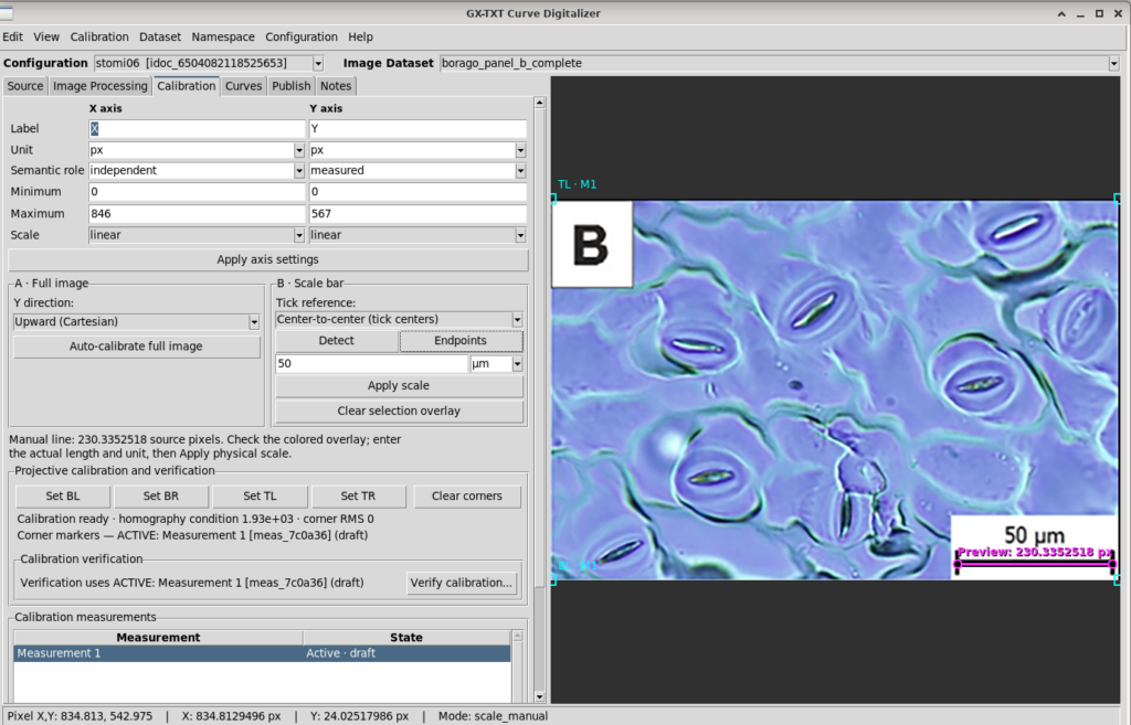
The measured distance was:

Giving the following conversion factor:

The scale was applied using Apply scale.

The calibration measurement was then accepted, reaching the Active · accepted state.

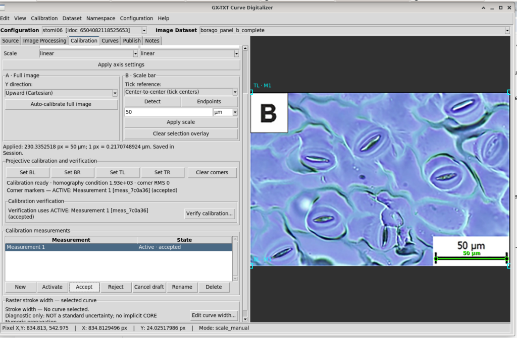
The numerical precision of the conversion factor should not be confused with measurement accuracy. Selecting the scale-bar endpoints and the quality of the image inevitably introduce uncertainty.

4. Preparing the image for digitization

Before digitizing the contours, we processed the image using Curve Digitalizer’s Image Processing tools.

The purpose was not to alter the dimensions of the structures, but to improve edge visibility.

The following settings were used:

Parameter	Value
Brightness/contrast	Enabled
Brightness	0.0
Contrast	39.0
Show processed preview	Enabled
Other visible filters	Disabled

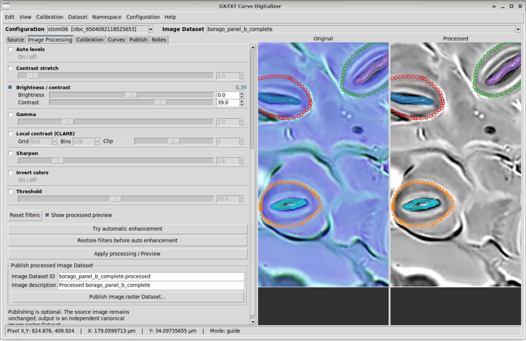
Being able to compare Original and Processed directly is particularly useful in this experiment.

Adjusting the contrast makes some boundaries easier to identify, but does not eliminate the ambiguities inherent in optical microscopy. In particular, blurred cell boundaries can make it difficult to define a unique outline.

Because the adjustment is photometric rather than geometric, the spatial calibration remains valid.

5. Digitizing the stomata

We selected four stomata that could be distinguished sufficiently well in the image.

Two independent outlines were acquired for each stoma:

Stoma	Outer boundary	Stomatal pore
01	stoma_01_outer	stoma_01_pore
02	stoma_02_outer	stoma_02_pore
03	stoma_03_outer	stoma_03_pore
04	stoma_04_outer	stoma_04_pore

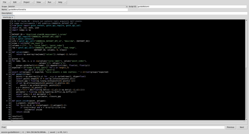
The outer outlines represent the selected boundary of the stomatal apparatus, whereas the inner outlines follow the edge of the central opening.

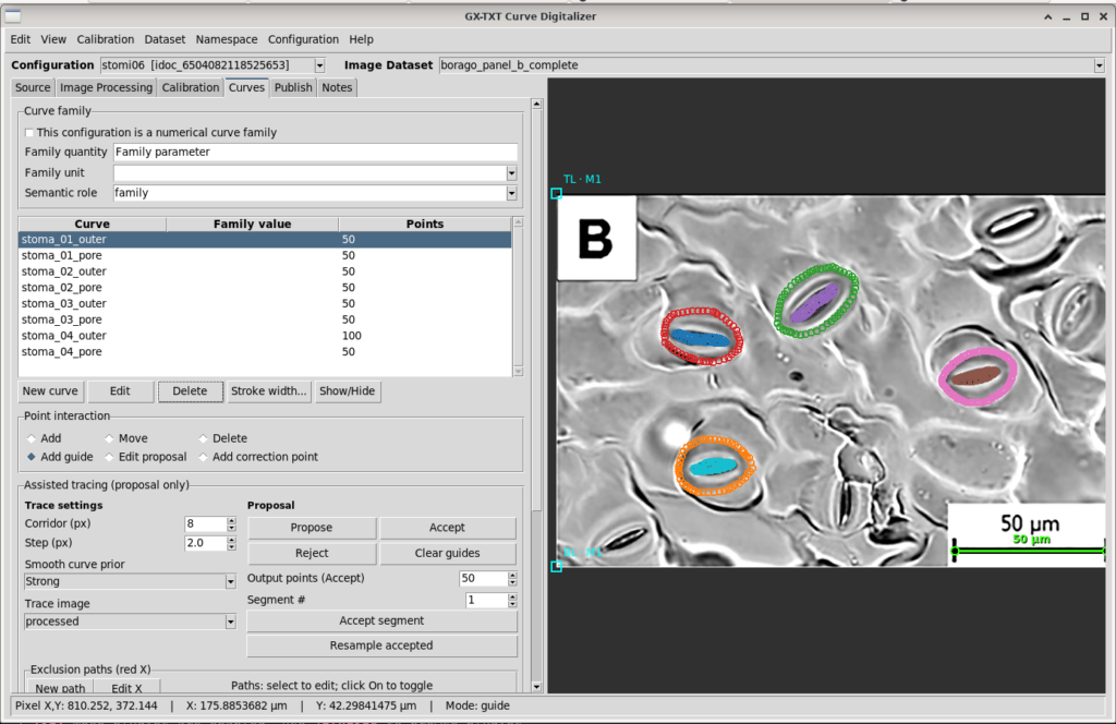
The dataset contains a total of 450 points:

• Seven curves with 50 points each.
• One curve, stoma_04_outer, with 100 points.

The points retain their insertion order. No monotonicity constraint was imposed.

This is necessary because a closed contour cannot be represented correctly simply by sorting points by their X coordinate.

Contour quality depends on edge visibility and the operator’s interpretation. A geometrically perfect trace cannot be guaranteed.

6. Publishing the dataset

After digitization, we selected the accepted calibration in the Publish tab and published the results.

The resulting Dataset is:

digitized.stomi06.measurement_1.curves

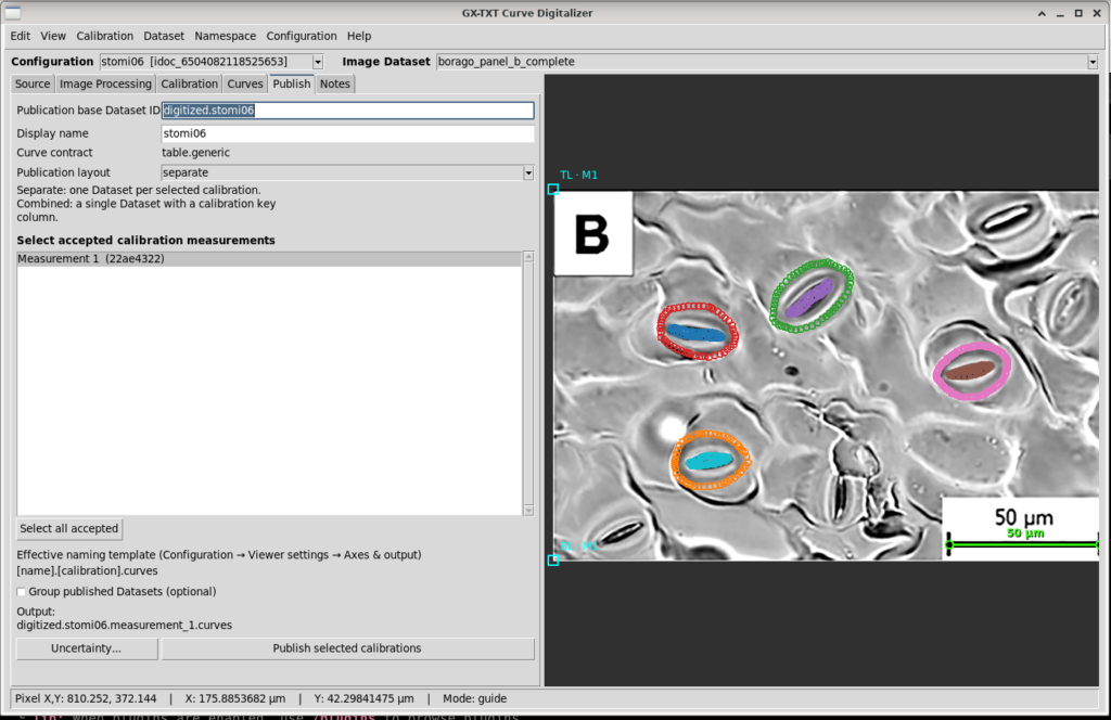
The Dataset contract is table.generic.

The published columns are:

Column	Meaning
x	X coordinate in µm
y	Y coordinate in µm
curve_id	Stable curve identifier
curve_label	Human-readable curve name
point_index	Point order within the curve
point_id	Point identifier
pixel_x	X coordinate in the original image
pixel_y	Y coordinate in the original image

Both the physical coordinates and the positions in the source image are therefore retained.

7. Analysis with the integrated Python editor

We used Python Script Workspace, which is already part of the framework, to perform the geometric analysis.

The stomata_06_user_contours.py script was registered in the session under the identifier guida06stomi, version 1.0.0.

The Dataset is accessed through the public GX-TXT client:

from gxtxt import (
    gxtxt_context,
    gxtxt_api_require,
    gxtxt_api_call,
)

dataset_id = "digitized.stomi06.measurement_1.curves"

gxtxt_api_require("CANONICAL_DATASET_API_v2@2")

metadata = gxtxt_api_call(
    "CANONICAL_DATASET_API_v2",
    "describe",
    [dataset_id],
)

To read the points, we can invoke read_range, using the Variable IDs actually associated with the coordinates and outlines.

The script groups coordinates by curve and sorts them by point_index.

Area calculation

For a closed polygonal contour, we apply the shoelace formula:

Perimeter calculation

The perimeter is obtained by summing the distances between consecutive vertices:

The script closes the contour numerically by connecting the final point to the first, without modifying the original Dataset.

For each stoma, the script then calculates the outer area, pore area, area obtained by subtraction, and ratio of the two areas.

Experimental results

Stoma	Outer area (µm²)	Pore area (µm²)	Area by subtraction (µm²)	Pore/outer area
01	324.43	22.29	302.14	6.87%
02	390.35	24.94	365.41	6.39%
03	329.38	24.99	304.38	7.59%
04	296.49	24.49	272.00	8.26%
Mean	335.16	24.18	—	7.28%

The calculated perimeters are:

Stoma	Outer perimeter (µm)	Pore perimeter (µm)
01	66.70	34.75
02	74.08	35.26
03	66.20	27.00
04	63.27	28.15

The sample standard deviation of the pore areas is 1.28 µm².

This value describes the spread of the measurements across the four outlines, not the uncertainty of any individual measurement.

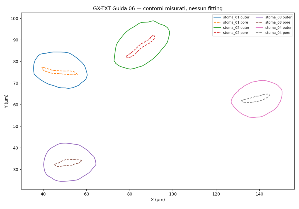
The script executed in the GX-TXT Python editor finished with PASS status and exit code 0.

8. Contour interpolation using splines

The digitized curves represent closed contours, for which a function of the form \(y=f(x)\) is generally unsuitable.

We therefore used a parametric representation:

The parameter \(t\) is defined from the cumulative chord lengths between vertices.

We used scipy.interpolate.CubicSpline to construct periodic cubic splines passing through the acquired points.

This analysis is implemented in the stomata_06_periodic_fit.py script.

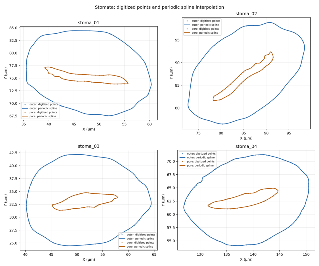
The interpolated representation provides smoother-looking contour visualization and allows the area of the original polygon to be compared with that of the interpolated curve.

Stoma	Contour	Polygon area (µm²)	Spline area (µm²)	Difference
01	Outer	324.4279	325.3744	+0.29%
01	Pore	22.2893	22.4751	+0.83%
02	Outer	390.3491	391.4748	+0.29%
02	Pore	24.9368	25.1435	+0.83%
03	Outer	329.3790	330.5078	+0.34%
03	Pore	24.9944	25.1140	+0.48%
04	Outer	296.4921	296.7113	+0.07%
04	Pore	24.4881	24.6059	+0.48%

The differences range from +0.07% to +0.83%.

This comparison describes the numerical effect of interpolation. It does not establish that the interpolated curve is anatomically more accurate than the digitized contour.

9. Using the public APIs from Python

An important aspect of the experiment is the ability to query scientific information already published by Curve Digitalizer.

There is no need to know the positions of the CSV columns in advance or rely solely on their names.

The GX-TXT documentation defines a dedicated public API:

CURVE_DIGITIZER_DATASET_SCHEMA_API_v1

This API maps semantic roles to the variables actually published.

In the version used for this experiment, it is directly accessible from the framework’s Tcl environment, but has not yet been registered as a direct call in the Python Script Bridge.

Python can nevertheless retrieve the published information indirectly by querying the public CORE APIs.

The relevant APIs are:

• DATASET_METADATA_API_v1
• DATASET_VARIABLE_SCHEMA_API_v3
• CANONICAL_DATASET_API_v2

An example query is:

from gxtxt import gxtxt_api_require, gxtxt_api_call

dataset_id = "digitized.stomi06.measurement_1.curves"

gxtxt_api_require("DATASET_METADATA_API_v1@1")
gxtxt_api_require("DATASET_VARIABLE_SCHEMA_API_v3@3")
gxtxt_api_require("CANONICAL_DATASET_API_v2@2")

metadata = gxtxt_api_call(
    "DATASET_METADATA_API_v1",
    "read",
    [dataset_id],
)

schema = gxtxt_api_call(
    "DATASET_VARIABLE_SCHEMA_API_v3",
    "list",
    [dataset_id],
)

description = gxtxt_api_call(
    "CANONICAL_DATASET_API_v2",
    "describe",
    [dataset_id],
)

The Curve Digitalizer Dataset contains metadata mapping roles such as curve_key, curve_name, and point_order to their actual Variable IDs.

Once these mappings have been retrieved and validated, Python can read the correct columns through the Canonical Dataset API.

The stomata_06_api_discovery.py file contains an exploratory example of this procedure, which still requires validation through a complete run in the editor.

Quality API

The CURVE_DIGITIZER_QUALITY_API_v2, by contrast, is directly available through the Python Script Bridge.

It can be used to query diagnostic information about the published points and curves.

For example:

from gxtxt import gxtxt_api_require, gxtxt_api_call
import json

gxtxt_api_require("CURVE_DIGITIZER_QUALITY_API_v2@2")

quality = gxtxt_api_call(
    "CURVE_DIGITIZER_QUALITY_API_v2",
    "diagnostics",
    [dataset_id],
)

report = json.loads(quality["report_json"])

for curve in report["curves"]:
    print(
        curve["curve_label"],
        curve["point_origins"],
    )

This API provides structural and diagnostic information, but does not certify contour accuracy.

Image Processing API

The CURVE_DIGITIZER_IMAGE_PROCESSING_API_v1 provides access to the processing operations and provenance of images that have been processed and published as Datasets.

In our experiment, the contrast adjustment was mainly used as a preview to facilitate digitization. This visual adjustment should not be confused with the publication of a new processed Image Dataset.

Calibration API

The CURVE_DIGITIZER_CALIBRATION_API_v1 exposes public Tcl methods for querying calibrations and geometric transformations.

Although it is not directly exposed through the Python Script Bridge in the version used, some published calibration information can be accessed indirectly via the CORE metadata APIs.

10. Metrological limitations and interpretation

The experiment demonstrates an acquisition and numerical-analysis workflow, but does not constitute a biologically validated morphometric measurement.

The outlines depend on micrograph quality, edge visibility, and the choices made by the operator during digitization.

Enhancing contrast makes the work easier but cannot recover anatomical information absent from the original image.

Spline interpolation is also a mathematical choice: it can produce a more continuous-looking contour without necessarily improving physical accuracy.

Four stomata selected from the same micrograph do not constitute independent biological replicates.

A more rigorous analysis would require a defined boundary-selection protocol, repeated assessments, and estimates of uncertainty in calibration and point positioning.

The difference between the outer area and pore area should also be interpreted as a planar geometric area, not automatically as the actual anatomical surface area of the guard cells.

11. Materials for reproducing the experiment

Conclusion

This guide demonstrates a complete acquisition and analysis workflow:

Optical micrograph → image preparation → micrometre-scale calibration → contour digitization → dataset publication → Python analysis → interpolated representation and geometric analysis.

The essential principle is the separation of responsibilities: Curve Digitalizer acquires and publishes the data, while the Python editor and the public GX-TXT APIs make it possible to analyze them scientifically.